Download
1 / 18
180 likes | 301 Views
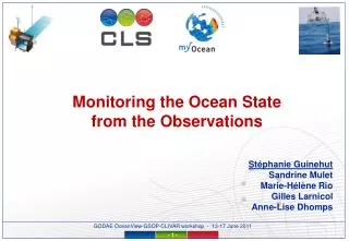
Monitoring the ocean from observations. Marie-Hélène Rio, Stéphanie Guinehut, Sandrine Mulet, Anne-Lise Dhomps , and Gilles Larnicol. OSTST, San Diego, 20 October 2011. Introduction. Our approach :

E N D
Monitoring the ocean from observations Marie-Hélène Rio, Stéphanie Guinehut, Sandrine Mulet, Anne-Lise Dhomps, and Gilles Larnicol OSTST, San Diego, 20 October 2011
Introduction • Our approach : • Consists of estimating 3D-thermohaline and current fields using ONLY observations and statistical methods • Represents a complementary approach to the one developed by forecasting centers – based on model/assimilation techniques • “Observation based” component of the Global MyOcean Monitoring and Forecasting Center lead by Mercator Océan • Previous studies have shown the capability of such approaches : • In producing reliable ocean state estimates (Guinehut et al., 2004; Larnicol et al., 2006) • In analyzing the contribution and complementarities of the different observing systems (in-situ vs. remote-sensing) (2nd GODAE OSE Workshop, 2009) OSTST, San Diego, 20 October 2011
The principle The observations The method The products Global 3D Ocean State [T,S,U,V,H] Weekly – 1993-2009 [0-1500m] 24 levels [1/3°] MyOcean V1 RT/RAN Altimeter, SST, winds, Geoid Guinehut et al., 2004 Guinehut et al., 2006 Larnicol et al., 2006 Rio et al., 2011 Mulet et al, submitted Intercomparison with independent data sets and model simulations Analysis of the ocean variability Observing System Evaluation T/S profiles, surface drifters OSTST, San Diego, 20 October 2011
Global T/S Armor3D - Method vertical projection of satellite data (SLA, SST) combination of synthetic and in-situ profiles 1 T(x,y,z,t) = (x,y,z,t).SLAsteric + (x,y,z,t).SST’ + Tclim (x,y,z,t) S(x,y,z,t)=’(x,y,z,t).SLAsteric + Sclim (x,y,z,t) 2 synthetic T(z), S(z) SLA, SST multiple linear regression 1 optimal interpolation 2 in-situ T(z), S(z) Armor3D T(z), S(z) OSTST, San Diego, 20 October 2011
Armor3D - 1993-2009 reanalysis NCEP Reynolds OI-SST 1/4° daily - 04/07/2007 SSALTO-DUACS MSLA 1/3° weekly DT - 04/07/2007 Synthetic T’ – at 100m Arivo climatology – July – T at 100 m OSTST, San Diego, 20 October 2011
Armor3D - 1993-2009 reanalysis In-situ observations – Coriolis data center Synthetic T’ – at 100m Armor3D T’ Argo T’ OSTST, San Diego, 20 October 2011
Armor3D - VALIDATION Rms error (% variance) in predicting subsurface T (left) and S (right) anomalies Independent T,S profiles Geographical distribution in 1°x1° boxes of 2002-2008 in-situ T and S profiles used for the validation, for a total of 3400 profiles. OSTST, San Diego, 20 October 2011
Global U/V/H Surcouf3D - Method Altimetry : Field of absolute geostrophic surface currents weekly - 1/3° Armor3D : 3D T/S fields weekly - 1/3° - [0-1500]m OSTST, San Diego, 20 October 2011
The CNES-CLS09 MDT Aviso maps of altimetric Sea Level Anomalies Argo, CTD T/S profiles 1993_2008 SVP drifting buoy velocities 1993_2008 cm cm cm/s CNES-CLS09 ¼° MDT MSS CLS01 – GRACE 400 km resolution cm OSTST, San Diego, 20 October 2011 Rio et al, 2011
Global U/V/H Surcouf3D - Method Altimetry : Field of absolute geostrophic surface currents weekly - 1/3° Armor3D : 3D T/S fields weekly - 1/3° - [0-1500]m In the following, unlessspecified, the synthetic T,S estimates are used Surcouf3D 3D geostrophic current fields weekly (1993-2008) 1/3° - 24 levels from 0 to1500m OSTST, San Diego, 20 October 2011
Surcouf3D - Comparison with model outputs • Vertical section at 60°W, in 2006 Thermal wind equation Reference level=1500m Vref=0m/s Surcouf3D at 500m Thermal wind equation Reference level=0m Vref=altimetry GLORYS at 500m GLORYS OSTST, San Diego, 20 October 2011
Surcouf3D - Validation • Comparison with RAPID current-meters in the Western boundary current off the Bahamas from April 2004 to April 2005 Florida Africa 26.5°North 76.5°West SURCOUF3D RAPID (current meters) GLORYS • Good correlation with independent obs., and with GLORYS OSTST, San Diego, 20 October 2011
Surcouf3D - Validation • Comparison with RAPID current-meters in the Western boundary current off the Bahamas from April 2004 to April 2005 Florida Africa 26.5°North 76.5°West Meridional velocities (cm/s) SURCOUF3D (synthetic T,S) RAPID (current meters) GLORYS RAPID (currentmeter at 100m + T,S using the thermal wind equation) SURCOUF3D (synthetic T,S) SURCOUF3D (synthetic T,S + Argo) RAPID (current meters) GLORYS • Importance of in-situ T/S profiles observations at depth for correctly resolving the inversion of the current OSTST, San Diego, 20 October 2011
Surcouf3D - AMOC variability at 25°N • Comparison with Bryden et al, 2005(section at 24.5° from Africa to 73°W and at 26.5°N off Bahamas) Floride Strait Transport from electrical cable (Bryden et al,2005) AMOC= Geost + Ekman + Florida (Surcouf3D, Bryden et al., 2005) Ekman Transport from wind stress ERAInterim Geostrophic Transport from 75°W to 15°W and from the surface to 1000m (Surcouf3D,Bryden et al., 2005) • Very consistent with Bryden et al, 2005 • Hight inter-annual variability • Hard to distinguish a long-term trend OSTST, San Diego, 20 October 2011
Surcouf3D - AMOC variability at 26.5°N • Comparison with RAPID and GLORYSfrom April 2004 to April 2009 • (monthly means + 12-month filtered) • Similar seasonal cycle • Amplitude differences ~ 10% • Higher variability in Surcouf than in Glorys • To be updated with recent RAPID measurements SURCOUF3D RAPID GLORYS OSTST, San Diego, 20 October 2011
Application – Mesoscale Vertical motion See Pascual et al. 2011 (poster OSTST) QG vertical velocitiy reanalysis 1993-2009 Pilot zone: Gulf Stream 3D fields Horizontal geostrophic currents from SURCOUF3D Upwelling (downwelling) upstream (downstream) of meander troughs Vertical velocities of the order of ±10 m/day. ~100 times larger than linear Ekman pumping. OSTST, San Diego, 20 October 2011
Application – Mesoscale Vertical motion See Pascual et al. 2011 (poster OSTST) Spatial mean Time mean High temporal correlation between EKE and w (magnitude) High spatial correlation between w and NPP (black box) OSTST, San Diego, 20 October 2011
Conclusions / Perspectives • All available observations of the ocean (satellite observations as SLA, SST, geoid and in-situ observations as T/S profiles and drifting buoy velocities) are merged to produce weekly 3D maps of Temperature, Salinity, and horizontal velocities from the surface to 1500m depth. • Armor3D/Surcouf3D reanalysis are distributed as part of the MyOcean project They are very useful : • to study the interannual variability of the hydrographic patterns, the AMOC … • to perform intercomparison exercices This will be continued in the future • The relevance and accuracy of the Armor3D/Surcouf3D estimates depends strongly on the existence of a complete (satellite + in-situ), homogeneous, and sustainable observations system OSTST, San Diego, 20 October 2011