Analyzing Coal Acidity Levels with Mixed Effects Model and ANOVA Table
This example outlines the use of a mixed effects model and ANOVA table to analyze the acidity levels of different coal samples. It includes testing for interactions and main effects, employing Tukey's procedure to identify significant differences, and formulating hypotheses of interest.

Analyzing Coal Acidity Levels with Mixed Effects Model and ANOVA Table
E N D
Presentation Transcript
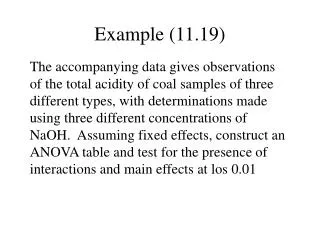
Example (11.19) The accompanying data gives observations of the total acidity of coal samples of three different types, with determinations made using three different concentrations of NaOH. Assuming fixed effects, construct an ANOVA table and test for the presence of interactions and main effects at los 0.01
Multiple Comparisons • * Use if HoAB is not rejected and either or both of HoA and HoB are rejected * • To test for differences of the i’s when HoA is rejected • Obtain Q,I,IJ(K-1) • Compute w = Q(MSE/(JK))1/2 • Order the from the smallest to largest and proceed with the underlining method
To test for differences of the j’s when HoB is rejected • Obtain Q,J,IJ(K-1) • Compute w = Q(MSE/(IK))1/2 • Order the from the smallest to largest and proceed with the underlining method
Example Cont’d (11.19) Use Tukey’s procedure to identify significant differences among the types of coal
Mixed Effects Model • The methods developed under mixed effects will naturally extend to the random effects model • Xijk = i + Bj + Gij + ijk • i = Fixed effect of Factor A at level I, i =0 • Bj = Random effect of Factor B at level j, Bj~N(0,B2)
Gij = Interaction effect of Factor A at level i and Factor B at level j , Gij ~ N(0 ,G2) • ijk = Random error of the kth observation with Factor A at level i and Factor B at level j
Hypotheses of Interest • HoA:1 = …. = I=0 ; HaA: at least one i 0 • HoB: B2 = 0 ; HaB: B2 > 0 • HoG: G2 = 0 ; HaB: G2 > 0 • * Test HoA and HoB only if HoG is not rejected*
Development of Test • Compute the Sums of Squares, Mean Squares, and ANOVA table identically to that under fixed effects • E[MSE] = 2 • E[MSA] = 2 + K G2 +(JK/I-1) i2 • E[MSB] = 2 + K G2 + IK B2 • E[MSAB] = 2 + K G2
Test of HoG • Fab= E[MSAB]/E[MSE] = (2 + K G2 )/ 2 • Under HoG: fab = 1 • Under HaG:fab = 1+(K G2 /2) > 1 for G2 >0 • Reject HoG if fab > F,(I-1)(J-1),IJ(K-1) • If we fail to reject HoG then test HoA and HoB
Test of HoA • FA = E[MSA]/E[MSAB] • = (2 + K G2 +(JK/I-1) i2)/(2 + K G2) • *Notice that the denominator of FA is E[MSAB]; not E[MSE]* • Under HoA: fA = 1 • Under HaA:fA = 1+ [(JK/I-1) i2)/(2 + K G2)] > 1 for i 0 • Reject HoA if fA > F,I-1,(I-1)(J-1)
Test of HoB • FB = E[MSB]/E[MSAB] • = (2 + K G2 + IK B2 )/(2 + K G2) • *Again the denominator of FB is E[MSAB]; not E[MSE]* • Under HoA: fB = 1 • Under HaA:fB = 1+[(IK B2 )/(2 + KG2)] > 1 for i 0 • Reject HoB if fB > F,J-1,(I-1)(J-1)
Example (11.19 modified) Assume that the determinations for the level of acidity of the three different types of coal were to made using 3 levels of a NaOH factor that could range between 0N and 1N. We randomly choose the concentrations .404N, .626N, and .786N