Download
1 / 20
200 likes | 288 Views
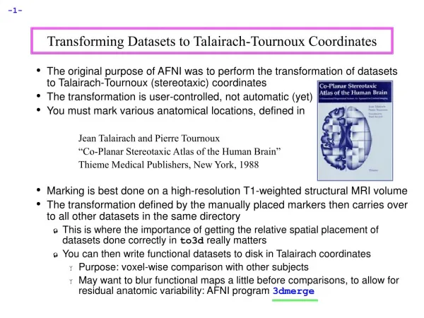
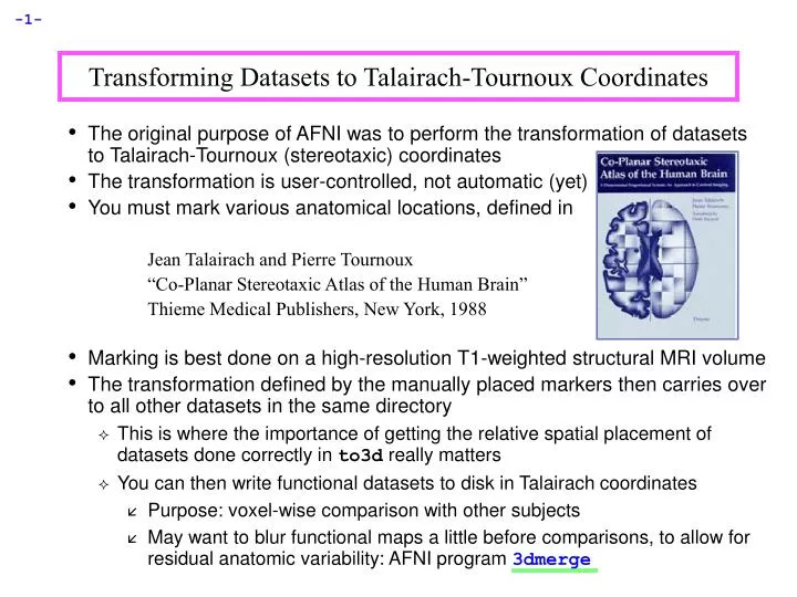
Transforming Datasets to Talairach-Tournoux Coordinates. The original purpose of AFNI was to perform the transformation of datasets to Talairach-Tournoux (stereotaxic) coordinates The transformation is user-controlled, not automatic (yet) You must mark various anatomical locations, defined in

E N D
Transforming Datasets to Talairach-Tournoux Coordinates • The original purpose of AFNI was to perform the transformation of datasets to Talairach-Tournoux (stereotaxic) coordinates • The transformation is user-controlled, not automatic (yet) • You must mark various anatomical locations, defined in Jean Talairach and Pierre Tournoux “Co-Planar Stereotaxic Atlas of the Human Brain” Thieme Medical Publishers, New York, 1988 • Marking is best done on a high-resolution T1-weighted structural MRI volume • The transformation defined by the manually placed markers then carries over to all other datasets in the same directory • This is where the importance of getting the relative spatial placement of datasets done correctly in to3d really matters • You can then write functional datasets to disk in Talairach coordinates • Purpose: voxel-wise comparison with other subjects • May want to blur functional maps a little before comparisons, to allow for residual anatomic variability: AFNI program 3dmerge
Transformation proceeds in two stages: • Alignment of AC-PC and I-S axes (to +acpc coordinates) • Scaling to Talairach-Tournoux Atlas brain size (to +tlrc coordinates) • Alignment to +acpc coordinates: • Anterior commissure (AC) and posterior commissure (PC) are aligned to be the y-axis • The longitudinal (inter-hemispheric or mid-sagittal) fissure is aligned to be the yz-plane, thus defining the z-axis • The axis perpendicular to these is the x-axis (right-left) • Five markers that you must place using the [Define Markers] control panel: AC superior edge = top middle of anterior commissure AC posterior margin = rear middle of anterior commissure PC inferior edge = bottom middle of posterior commissure First mid-sag point = some point in the mid-sagittal plane Another mid-sag point = some other point in the mid-sagittal plane • This procedure tries to follow the Atlas as precisely as possible • Even at the cost of confusion to the user (e.g., you)
Press this IN to create or change markers [Define Markers] Color of “primary” (selected) marker Color of “secondary” (not selected) markers Size of markers (pixels) Size of gap in markers Select which marker you are editing Clear (unset) primary marker Set primary marker to current focus location Carry out transformation to +acpc coordinates Perform “quality” check on markers (after all 5 are set)
Class Example - Selecting the ac-pc markers: • cd AFNI_data1/demo_tlrc Descend into the demo_tlrc/ subdirectory • afni & This command launches the AFNI program • The “&” keeps the UNIX shell available in the background, so we can continue typing in commands as needed, even if AFNI is running in the foreground • Select dataset anat+orig from the [Switch Underlay] control panel The AC-PC markers appear only when the orig view is highlighted Press IN to view markers on brain volume • Select the [Define Markers]control panel to view the 5 markers for ac-pc alignment • Click the [See Markers] button to view the markers on the brain volume as you select them • Click the [Allow edits] button in the ac-pc GUI to begin marker selection
First goal is to mark top middle and rear middle of AC • Sagittal: look for AC at bottom level of corpus callosum, below fornix • Coronal: look for “mustache”; Axial: look for inter-hemispheric connection • Get AC centered at focus of crosshairs (in Axial and Coronal) • Move superior until AC disappears in Axial view; then inferior 1 pixel • Press IN [AC superior edge] marker toggle, then [Set] • Move focus back to middle of AC • Move posterior until AC disappears in Coronal view; then anterior 1 pixel • Press IN [AC posterior margin], then[Set]
Second goal is to mark inferior edge of PC • This is harder, since PC doesn’t show up well at 1 mm resolution • Fortunately, PC is always at the top of the cerebral aqueduct, which does show up well (at least, if CSF is properly suppressed by the MRI pulse sequence) cerebral aqueduct • Therefore, if you can’t see the PC, find mid-sagittal location just at top of cerebral aqueduct and mark it as[PC inferior edge] • Third goal is to mark twointer-hemispheric points (above corpus callosum) • The two points must be at least 2 cm apart • The two planes AC-PC-#1 and AC-PC-#2 must be no more than 2o apart
Once all 5 markers have been set, the [Quality?] Button is ready • You can’t [Transform Data] until [Quality?] Check is passed • In this case, quality check makes sure two planes from AC-PC line to mid-sagittal points are within 2o • Sample below shows a 2.43o deviation between planes ERROR message indicates we must move one of the points a little • Sample below shows a deviation between planes at less than 2o. Quality check is passed • We can now save the marker locations into the dataset header
When [Transform Data] is available, pressing it will close the [Define Markers] panel, write marker locations into the dataset header, and create the +acpc datasets that follow from this one • The [AC-PC Aligned] coordinate system is now enabled in the main AFNI controller window • In the future, you could re-edit the markers, if desired, then re-transform the dataset (but you wouldn’t make a mistake, would you?) • If you don’t want to save edited markers to the dataset header, you must quit AFNI without pressing [Transform Data] or [Define Markers] • ls The newly created ac-pc dataset, anat+acpc.HEAD,is located in our demo_tlrc/ directory • At this point, only the header file exists, which can be viewed when selecting the [AC-PC Aligned] button • more on how to create the accompanying .BRIK file later…
Scaling to Talairach-Tournoux (+tlrc) coordinates: • We now stretch/shrink the brain to fit the Talairach-Tournoux Atlas brain size (sample TT Atlas pages shown below, just for fun)
Class example - Selecting the Talairach-Tournoux markers: • There are 12 sub-regions to be scaled (3 A-P x 2 I-S x 2 L-R) • To enable this, the transformed +acpc dataset gets its own set of markers • Click on the [AC-PC Aligned] button to view our volume in ac-pc coordinates • Select the [Define Markers] control panel • A new set of six Talairach markers will appear: The Talairach markers appear only when the AC-PC view is highlighted
Using the same methods as before (i.e., select marker toggle, move focus there, [Set]), you must mark these extreme points of the cerebrum • Using 2 or 3 image windows at a time is useful • Hardest marker to select is [Most inferior point] in the temporal lobe, since it is near other (non-brain) tissue: Sagittal view: most inferior point Axial view: most inferior point • Once all 6 are set, press [Quality?] to see if the distances are reasonable • Leave [Big Talairach Box?] Pressed IN • Is a legacy from earliest (1994-6) days of AFNI, when 3D box size of +tlrc datasets was 10 mm smaller in I-direction than the current default
Once the quality check is passed, click on [Transform Data] to save the +tlrc header • ls The newly created +tlrc dataset, anat+tlrc.HEAD,is located in our demo_tlrc/ directory • At this point, the following anatomical datasets should be found in our demo_tlrc/ directory: anat+orig.HEAD anat+orig.BRIK anat+acpc.HEAD anat+tlrc.HEAD • In addition, the following functional dataset (which I -- the instructor -- created earlier) should be stored in the demo_tlrc/ directory: func_slim+orig.HEAD func_slim+orig.BRIK • Note that this functional dataset is in the +orig format (not +acpc or +tlrc)
Automatic creation of “follower datasets”: • After the anatomical +orig dataset in a directory is resampled to +acpc and +tlrc coordinates, all the other datasets in that directory will automatically get transformed datasets as well • These datasets are created automatically inside the interactive AFNI program, and are not written (saved) to disk (i.e., only header info exists at this point) • How followers are created (arrows show geometrical relationships): anat+orig anat+acpc anat+tlrc func+orig func+acpc func+tlrc • In the class example, func_slim+orig will automatically be “warped” to our anat dataset’s ac-pc (anat+acpc) & Talairach (anat+tlrc) coordinates • The result will be func_slim+acpc.HEAD and func_slim+tlrc.HEAD, located internally in the AFNI program (i.e., you won’t see these files in the demo_tlrc/ directory) • To store these files in demo_tlrc/, they must be written to disk. More on this later…
How does AFNI actually create these follower datsets? • After [Transform Data] creates anat+acpc, other datasets in the same directory are scanned • AFNI defines the geometrical transformation (“warp”) from func_slim+orig using the to3d-defined relationship between func_slim+orig and anat+orig, AND the markers-defined relationship between anat+orig and anat+acpc • A similar process applies for warpingfunc_slim+tlrc • These warped functional datasets can be viewed in the AFNI interface: Functional dataset warped to anat underlay coordinates func_slim+orig “func_slim+acpc” “func_slim+tlrc” • Next time you run AFNI, the followers will automatically be created internally again when the program starts
“Warp on demand” viewing of datasets: • AFNI doesn’t actually resample all follower datasets to a grid in the re-aligned and re-stretched coordinates • This could take quite a long time if there are a lot of big 3D+time datasets • Instead, the dataset slices are transformed (or warped) from +orig to +acpc or +tlrc for viewing as needed (on demand) • This can be controlled from the [Define Datamode] control panel: If possible, lets you view slices direct from dataset .BRIK If possible, transforms slices from ‘parent’ directory Interpolation mode used when transforming datasets Grid spacing to interpolate with Similar for functional datasets Write transformed datasets to disk Re-read: datasets from current session, all session, or 1D files Read new: session directory, 1D file, dataset from Web address Menus that had to go somewhere AFNI titlebar shows warp on demand: {warp}[A]AFNI2.56b:AFNI_sample_05/afni/anat+tlrc
Writing “follower datasets” to disk: • Recall that when we created anat+acpc and anat+tlrc datasets by pressing [Transform Data], only .HEAD files were written to disk for them • In addition, our follower datasets func_slim+acpc and func_slim+tlrc are not stored in our demo_tlrc/ directory. Currently, they can only be viewed in the AFNI graphical interface • Questions to ask: • How do we write our anat.BRIK files to disk? • How do we write our warped follower datasets to disk? • To write a dataset to disk (whether it be an anat .BRIK file or a follower dataset), use one of the [Define Datamode]Write buttons: ULay writes current underlay dataset to disk OLay writes current overlay dataset to disk Manywrites multiple datasets in a directory to disk
Class exmaple - Writing anat (Underlay) datasets to disk: • You can use [Define Datamode]Write[ULay] to write the current anatomical dataset .BRIK out at the current grid spacing (cubical voxels), using the current anatomical interpolation mode • After that, [View ULay Data Brick] will become available • ls to view newly created .BRIK files in the demo_tlrc/ directory: anat+acpc.HEAD anat+acpc.BRIK anat+tlrc.HEAD anat+tlrc.BRIK • Class exmaple - Writing func (Overlay) datasets to disk: • You can use [Define Datamode]Write[OLay] to write the current functional dataset .HEAD and BRIK files into our demo_tlrc/ directory • After that, [View OLay Data Brick] will become available • ls to view newly resampled func files in our demo_tlrc/ directory: func_slim+acpc.HEAD func_slim+acpc.BRIK func_slim+tlrc.HEAD func_slim+tlrc.BRIK
Command line program adwarp can also be used to write out .BRIK files for transformed datasets: adwarp -apar anat+tlrc -dpar func+orig • The result will be: func+tlrc.HEAD and func+tlrc.BRIK • Why bother saving transformed datasets to disk anyway? • Datasets without .BRIK files are of limited use: • You can’t display 2D slice images from such a dataset • You can’t use such datasets to graph time series, do volume rendering, compute statistics, run any command line analysis program, run any plugin… • If you plan on doing any of the above to a dataset, it’s best to have both a .HEAD and .BRIK files for that dataset
Some fun and useful things to do with +tlrc datasets are on the 2D slice viewer Buttton-3 pop-up menu: • [Talairach to] Lets you jump to centroid of regions in the TT Atlas (works in +orig too)
[Where am I?] Shows you where you are in the TT Atlas (works in +orig too) • [Atlas colors] Lets you display color overlays for various TT Atlas-defined regions, using the Define Function See TT Atlas Regions control (works only in +tlrc)