Download
1 / 58

E N D
Neural Network(NN) “A neural network is an interconnected assembly of simple processing elements units or nodes, whose functionality is loosely based on the animal neuron. The processing ability of the network is stored in the interunit connection strengths, or weights, obtained by a process of adaptation to, or learning from, a set of training patterns.” Neural network is to obtain a model of weighting for a good prediction of an output based on a profile of input parameter.
NN can be supervised or unsupervised For example, during training, we indicate a correct output for customers that have taken advantage of pervious promotions as 1 for the first output node and 0 for the second output node. Once trained, the NN will recognize a node 1, node 2 output combination of 0.9, 0.2 as a new customer likely to take advantage of a promotion. The purpose of changing the connection weights is to minimize training set error rate.
Backpropagation Learning Algorithm Backpropagation algorithm is a learning algorithm applied to multilayer feedforward networks. During the training phase, training samples are sequentially presented to the network. These inputs are propagated forward layer by layer until a final output is computed. By comparing the final output to the target output of the corresponding sample, errors are computed. These errors act as feedbacks for the adjustment of the weights and biases layer by layer in a backward direction. Backpropagation is a learning technique that adjusts weights in the NN by propagating weight changes backward from the sink to the source nodes.
Backpropagation Learning Algorithm Backpropagation learns using a method of gradient descent to search for a set of weights that can model the given classification problem so as to minimize the mean squared distance between the network’s class prediction and the actual class label of the samples.
Backpagation Algorithm Progapation (N, X) E = (1/2) ∑ (Di – Yi)2 Gradient (N’, E) where N = starting neural network X = input tuple from training set D = output tuple desired Gradient = slope of error function descent N’ = improved neural network E = error rate
Mean Squared Error (MSE) MSE = (Yi – Di)2 2 Where Di are output tuple desired Yi are computed output
Transfer Function Sigmoid function is one of the common transfer functions used for Backpropagation to enforce output (target) value ranges from 0.0 to 1.0. f (x) = _______1_____ ( 1 + e-x )
Wji = -ŋ (dE)= - ŋ (dE) (dyi)(dSi) dW dyi dSi dWji Where ŋ = learning rate, S = transfer function, E = error rate dyi = d ( 1 ) = (1 - 1 ) ( 1 ) = (1 – yi) yi dSi dSi 1 + e-Si 1 + e-Si 1 + e-Si Where e = 2.718 dSi = yj dWji dE = d ( 1 Σ(dm – ym)2) = - (di – yi) dyi dyi 2 Wji= ŋ yj (1-yi) (di-yi)yi = ŋ Ej yi where Ej = yj (1-yi) (di-yi) as a new error rate Therefore
NN Backpropagation Learning algorithm processing steps Step 1: Separate the dataset into training and testing sets Step 2: Select the Neural network topology (to decide number of hidden layer, too many may be over fiting, too few may be no convergence) Step 3: Set the parameters of the network Step 4: Training the network Step 5: Testing the network Step 6: Repeat the above step(s) if required
Step 4. 1 Compute Output nodes value Submit training set & compute layers’ responses Ij =Σi Wij Oi +θj Oj=1 / (1 + e –Ij; ) where Ij is output node value before transfer function Oj is the output node value after transfer function θj is the bias value of difference between estimated value and the actual value Wij is the weight value to output node
Step 4.2 & 4.3 Compute errors between derived value and training data value in output and hidden node nodes Compute errors Ej of output node Oj : Ej = Oj (1 - Oj )( Tj - Oj ) Where T = training data value Compute errors Ej of hidden node Oj by backpropagation Ej = Oj (1 - Oj ) Σk Ek Wjk Where Ek is the computed error in output node
Step 4.4 Compute modified weights of Neural Network modeling values Update the weights of the hidden nodes: Wij = Wij + (η) Ej Oi ; Where η is the learning rate Ei is the derived error Oi is the node value
Step 4.5 Update Bias θj = θj + ∆θj of which ∆θj = (η) Ej
Initialize weights & biases Start with a new training sample Submit training set & compute layers’ responses Oj=1 / (1 + e –Ij; )of which Ij =Σi Wij Oi +θj Update the weights of output layer: Wij = Wij + ∆Wij of which ∆Wij = (η) Ej Oi ; Ej = Oj (1 - Oj )( Tj - Oj ) Y Update the weights of the hidden layer: Wij = Wij + ∆Wij of which ∆Wij = (η) Ej Oi ; Ej = Oj (1 - Oj ) Σk Ek Wjk Step 4.7 Check the terminating condition: No. of Epoch run < pre-determined level N N STOP Update the biases: θj =θj +∆θj of which∆θj = (η) Ej N Step 4.6 Check the terminating condition: Total error pre-determined level Calculate the error generated from each sample Y N STOP Calculate Total error generated from each Epoch Any samples in the training set ? Y N Start a new Epoch Training the Network
Processing Elements Processing Element W1 W2 W3 X1 X2 X3 Summation function Transfer function Y θ ∑
Step (3): Initialize the weights and biases The weights (W) and the biases (θ) are initialized to small random numbers (e.g. ranging from –1.0 to 1.0, or –0.5 to 0.5).
Step (4.1) : Propagate the inputs forward The training sample is fed to the input layer of the network. To compute the net input to each unit in a hidden layer or output layer, each input connected to the unit is multiplied by its corresponding weight, and this is summed. Ij = Σi Wij Oi +θj where Wij is the weight of the connection from unit i in the previous layer to unit j; Oi is the output of unit i from the previous layer; andθj is the bias of the unit. Each unit takes its net input and applies an activation function to it. Sigmoid function is chosen as activation function. The output of unit j is computed as Oj = 1 / ( 1 + e –Ij )
Step (4.2): Backpropagate steps: Weights and biases modification The weights and biases are updating backwards, i.e. from the output layer back to the hidden layers and finally to the input layer. For a unit j in the output layer, Ej is computed as: Ej = Oj (1 - Oj )( Tj - Oj ) where Oj is the actual output of unit j, and Tj is the true output observed from the training sample
Step 4.3, 4.4 & 4.5 In case the unit j is in the hidden layer unit, Ej is computed by Ej = Oj (1 - Oj ) Σk Ek Wjk Where Wjk is the weight of the link from “node j” to “node k” in the next higher layer. Weights are updates as follows: Wij = Wij + ∆Wij where ∆Wij = (η) Ej Oi, of which “η” is the learning rate, a constant typically having a value between 0.0 and 1.0 Biases are updated as follows θj = θj + ∆θj where ∆θj = (η) Ej, of which “η” is the learning rate
Step 4.6: Check Terminating Condition (1) The difference between Total Errors of two consecutive Epoch is smaller than a pre-determined level. Mean Square Error: E = 1/N(Σj( Tj - Oj )2), where N is the number of output nodes, Oj is the value of output node j computed from the network, and Tj is the target output of the corresponding node observed from the training sample. Total Error of the network is the sum of errors of all samples, i.e. TE = Σp (1/N)(Σj( Tj - Oj )2), where p is the number of samples in the training set; (2) Percentage of samples misclassified in the previous Epoch is below a pre-determined value Percentage of samples misclassified = [(Number of misclassified samples) / (Total number of samples)] * 100%. This terminating condition is applicable for classification problem. (3) A pre-specified number of Epoch has been finished, say, 1,000 iterations.
Step 5: Compute the Total Error There are different formulas for calculating Total Error. For classification problem, the formula: [Number of misclassified samples] ------------------------------------------ * 100% (Total number of samples) Can be applied
An example of computing Backpropagation algorithm w14 O1=1 11 w15 O4 w46 41 O6=1 O2=0 21 61 W25 w56 O5 51 W35 O3=0 31 Steps 1 & 2 Applying Backpropagation algorithm W15 W24 W34
Copy final weights & biases of trained network Start with a new testing sample Submit testing set & compute layers’ responses: Oj = 1 / ( 1 + e –Ij; ) of which Ij = Σi Wij Oi +θj ; Calculate the error generated from each sample: (error increases by one if the sample is misclassified) Calculate Total error generated from the whole training set: (Total error can be the percentage of samples misclassified) Any samples in the testing set ? Y N STOP Step 5: Testing the Network
Step (5): Copy the weights and biases from the trained network The final weights and biases of the network obtained from the training stage are used in the testing stage and these values are maintained unchanged during the whole testing stage.
Step (5): Pass the samples in testing set to the network Each sample in the testing set is to be fed in the network for testing purpose until the end of the dataset.
Step (5): Compute the total error Formula applied to calculate Total error in the testing stage should be the same as the one applied in the training stage.
Case study of using NN backpropagation learning algorithm Sales trend forecast is a very important issue for retailing industry. Traditionally, past sales information can be collateral provided as the basic predict criteria. Moreover, fraud detection on sales figures, etc… will cause the inaccurate of the prediction on sales. The use of KDD can be used for the supplement of the traditional techniques in sales prediction to prevent fraud and wrong data entry. This case study applies the KDD process for categorizing sales trend prediction as either good (good sales in future) or bad (sales will be not good in future).
Step 1 data selection An ideal training set is one with similar distribution among each possible outcome. In this case study, 55,000 samples are randomized and then divided into two groups: 27,500 samples for good sales trend and 27,500 samples for bad sales trend. A sample is classified as “good sales trend” if the value of the output node is 0.8 or above, otherwise, below 0.2 is classified as “bad sales trend”. It is considered as non-classified if the output value is between 0.21 and 0.79.
Step 1 Data Sources • Attribute Name Data Type Description Coding • 1 Brand C brands the company has A11: GM (G Men) • A12: GL (G Ladies) • A13: UM (U Men) • A14: UL (U Ladies) • A15: UW (U Women) • 2 Category C category of the product A21: Blazer • A22: Shirt • A23: Pant • A24: Tee • A25: Jacket • A26: Skirt • A27: Trouser • A28: Coat • A29: Tie • A210: Bag • A211: Belt • A212: Sweater • A213: Sock • 3 Story C story of the product A31: BS (Basic) • A32: CD (Classification) • A33: TD (Trendy)
Step 1 Data Sources • 4 Fabric C fabric of the product A41: Cotton • A42: Wool / Cashmere • A43: Polyester • A44: Nylon • A45: Leather • A46: Spandex / Lycra • A47: Silk • 5 Fabric Type C fabric type of the product A51: Knit • A52: Woven • A53: Others • 6 Color C color of the product A61: 00 -10 • A62: 11 – 20 • A63: 21 – 30 • A64: 31 – 40 • A65: 41 – 50 • A66: 51 – 60 • A67: 61 – 70 • A68: 71 – 80 • A69: 81 – 90 • A610: 91 - 99 • 7 Price C retail price of the product A71: 0 – 100 • A72: 101 – 200 • A73: 201 – 400 • A74: 401 – 600 • A75: 601 – 800 • A76: 801 – 1000 • A77: Above 1000
Step 1 Data Sources • 8 Shop location C Shop location A81: Kwai Tsing • A82: Tsuen Wan • A83: Causeway Bay • A84: Central • A85: Westean District • A86: Mong Kok • A87: Tsim Sha Tsui • A88: Kowloon Bay • A89: Tuen Mun • A810: Yuen Long • A811: Shatin • A812: Eastern District • A813: Hung Hom • A814: Jordan • A815: Ma On Shan • A816: New Territeries • A817: Diamond Hill • A818: Southern District • A819: Sham Shui Po • 9 District C Shop District A91: HK Island • A92: Kowloon • A93: New Territories • 10 Chain C Brand chain A101: U • A102: G • 11 Gender C Brand gender A111: M (Male) • A112: F (Female) • A113: K (Kid)
Data type Description Coding Result C To distinguish the sales into either ‘good’ or ‘bad’ 1 : Good 0 : Bad Step 1 Target class data for prediction In addition to the above-mentioned 11 attributes, there is a field (the last field) records the class of a sample belong to.
Step 1 Data Coding Since category data type is used in the dataset, it is necessary to transform the data into appropriate formats for Neural Network, i.e. 0 or 1. ‘One of N’ coding is applied in this dissertation. One separate input node will be assigned to each category in an attribute. The input node value is ‘1’ when the category is selected; otherwise, ‘0’ will be given as its value. E.g. for Attribute 1 - Brand, it has 5 nodes (A11: GM, A12: GL, A13: UM, A14: UL, A15: UW). If A11 is chosen, the inputs nodes of them are (1, 0, 0, 0, 0). All the transformed data are stored in SAMPLE table.
Step 1 Sample Table Encoding = original value – minimal value maximal value = minimal value A11 A12 A13 A14 A15 A21 A22 A23 A24 A25 A26 A27 A28 A29 A210 A211 A212 A213 A31 1 0 0 0 0 0 1 0 0 0 0 0 0 0 0 0 0 0 1 1 0 0 0 0 0 1 0 0 0 0 0 0 0 0 0 0 0 1 1 0 0 0 0 0 1 0 0 0 0 0 0 0 0 0 0 0 1 1 0 0 0 0 0 1 0 0 0 0 0 0 0 0 0 0 0 0
Step 1 Sample Table A32A33 A41 A42 A43 A44 A45 A46 A47 A51 A52 A53 A61 A62 A63 A64 A65 A66 A67 A68 0 0 0 0 0 0 1 0 0 0 1 0 0 0 0 0 1 0 0 0 0 0 0 0 1 0 0 0 0 0 1 0 0 1 0 0 0 0 0 0 0 0 1 0 0 0 0 0 0 0 1 0 0 0 1 0 0 0 0 0 1 0 1 0 0 0 0 0 0 0 1 0 1 0 0 0 0 0 0 0
Step 1 Sample table A69A610 A71 A72 A73 A74 A75 A76 A77 A81 A82 A83 A84 A85 A86 A87 A88 A89 A810 0 0 0 1 0 0 0 0 0 0 0 0 0 0 0 0 0 0 0 0 0 1 0 0 0 0 0 0 0 0 0 0 0 0 0 0 0 0 0 0 0 1 0 0 0 0 0 0 0 0 0 0 0 0 0 0 0 0 0 1 0 0 0 0 0 0 0 0 0 0 0 0 0 0 0 0
Step 1 Sample table A811 A812 A813 A814 A815 A816 A817 A818 A819 A91 A92 A93 A101 A102 A111 A112 A113 RESULT 0 0 0 0 1 0 0 0 0 0 1 0 0 1 1 0 0 0 0 0 0 0 1 0 0 0 0 0 1 0 0 1 1 0 0 1 0 0 0 0 1 0 0 0 0 0 1 0 0 1 1 0 0 1 0 0 0 0 1 0 0 0 0 0 1 0 0 1 1 0 0 1
Step 2 & 3 75-30-1 network is presented as an example: 75 input nodes NI[0], NI[1], ..., NI[75] 30 hidden nodes NH[0], NH[1], ..., NH[29] 1 output node NO 2250 weights between input layer and hidden layer (WI[i][j] represents the weight for the link between NI[i] and NH[j]) WI[0][0], WI[0][1], ...,WI[0][29], WI[1][0], WI[1][1], ..., W[1][29], s s WI[74][0], WI[74][1], ..., WI[74][29] 30 weights between hidden layer and output layer WO[0], WO[1], ..., WO[29] 30 biases attached to the hidden nodes BI[0], BI[1], ..., BI[29] 1 bias attached to the output node BO
Step 4 Training the network Error Rate of the networks__________ Epoch 75 – 10 – 1 75 – 30 – 1 75 – 50 - 1 1 50.00% 49.75% 50.00% 5 45.98% 43.84% 42.76% 10 39.07% 36.25% 34.82% 20 28.87% 22.12% 20.41% 40 14.76% 7.07% 6.79% 60 5.40% 2.52% 3.05% 80 2.99% 2.21% 2.16% 100 2.13% 1.98% 1.93%