Chase & Backchase: A Versatile Tool for Query Optimization
Chase & Backchase: A Versatile Tool for Query Optimization. Lucian Popa , Alin Deutsch, Arnaud Sahuguet, Val Tannen University of Pennsylvania. Logical vs. Physical. Unfortunately, limited cooperation !. A separation is necessary for physical data independence:. Network. Logical schema.

Chase & Backchase: A Versatile Tool for Query Optimization
E N D
Presentation Transcript
Chase & Backchase:A Versatile Tool for Query Optimization Lucian Popa, Alin Deutsch, Arnaud Sahuguet, Val Tannen University of Pennsylvania
Logical vs. Physical Unfortunately, limited cooperation ! • A separation is necessary for physical data independence: Network Logical schema Physical schema Physical optimization Logical optimization
Optimization Techniques Traditional More “exotic” • Some rewriting (unnesting) • Acces path (index) use (ad-hoc) • Join ordering (dynamic programming) • Semantic optimization (more rewriting) • Use of materialized views (rewriting, too) • Object-oriented techniques(everything above, but OO! ) Logical Physical Physical Logical Both ?! Mixed • Limited cooperation, so far, because of : • different foundations • different affiliation: logical or physical
Bridges Use of materialized views • What is needed: interaction between all these techniques. • can produce better plans, by enabling each other: • This work connects together some of these techniques, by finding a common foundation Semantic optimization Use of indexes
In a (Coco)Nutshell • The Unifier: Constraints (Dependencies): • logical constraints: • semantic relationships among elements of the logical schema • physical constraints: • semantic relationships between elements of the physicalschema and elements of the logical schema • Chase with constraints produces the universal plan UP: • UP incorporates all relevant access paths • subqueries of UP provide the search space (candidate plans) • Backchase: • search among candidate plans for scan-minimal queries, checking for equivalence using (reverse) chase • search space can be pruned using cost-based optimization
Talk Outline • Motivation and Overview • Logical and Physical Constraints, Chase and Backchase (VLDB’99) • Theoretical Results (ICDT’99, VLDB’99, recent improvements) • Using Cost Information • Experimental Results (SIGMOD’00, recent improvements) • Conclusion
fresh base type for oids Dept : Dict < Doid, Struct { string DName; Set <string> DProjs; }> Logical Schema (ODMG syntax) Proj : Set < Struct { string PName; string PDept; string CustName; string Budget;} > class Dept (extent depts){ attribute string DName; attribute Set<string> DProjs;} • To formally describe classes and their operations: use dictionaries (finite functions).
Translating OO Queries into Dictionary Form selectstruct(PN: s, DN: d.DName) from depts d , d.DProjs s OO selectstruct(PN: s, DN: Dept [d].DName) fromdomDept d , Dept [d].DProjs s Dict “domain” as extent “lookup” for oid dereferencing • Dictionary operations: dom M, M[k] • Constraints are translated in a similar way
Logical Schema Constraints • Describe semantic relationships among elements of the logical schema • Example: an inverse relationship between Proj and Dept: (RIC1) (d domDept) (sDept [d].DProjs) (p Proj) s = p.PName (INV2) (p Proj) (d domDept) p.PDept = Dept [d].DName (s Dept [d].DProjs)p.Pname = s + two others …
Physical Schema • Two indexes for relation Proj : Primary Index on PNameI : Dict <string, T> Secondary Index on CustNameSI : Dict <string, Set < T >> (where T is the type of tuples in Proj) • A materialized view (a la “join index”) : • JI : Set< Struct{DoidJDoid; string JPN} > • JI = select struct (JDoid: d, JPN: p.PName) • fromdomDept d, Dept [d].DProjs s, Proj p • where s = p.PName
Physical Schema Constraints Describe semantic relationship between elements of the logical schema and elements of the physical schema. One of the constraints for SI : • (SI1) (p Proj) (k domSI) • (t SI[k]) [ k = p.CustName andp = t ] • One of the constraints for JI : • (JI1) (d domDept) (s Dept [d].DProjs) (p Proj) • [ s = p. PName • • ( j JI) j.JDoid = dand j.JPN = p.Pname • ]
An Example of Interaction in Optimization A user (logical) query selectstruct(PN: s, PB: p.Budg, DN: Dept [d].DName) fromdomDept d, Dept [d].DProjs s , Proj p where s = p.PName and p.CustName = “CitiBank” • The query is chased with all the applicable logical and physical constraints (eg., RIC1, SI1, JI1) • The result of the chase is the universal plan.
The Generalized Chase distinct! distinct! selectO(r1,…,rm) from R1r1,…,Rmrm, S1s1,…,Snsn where B1(r1,…,rm)and B2(r1,…,rm,s1,…,sn) d Let d be the constraint: (r1R1) … (rmRm) [B1(r1,…,rm) (s1S1) … (snSn) B2(r1,…,rm,s1,…,sn) ] selectO(r1,…,rm) from R1r1,…,Rmrm where B1(r1,…,rm)
A Universal Plan Added by chase selectstruct(PN: s, DN: Dept [d].DName) fromdomDept d , Dept [d].DProjs s , Proj p, JI j, dom SI k, SI [k] t, dom I i where s = p.PNameand p.CustName = “CitiBank” andDept[d].DName = p.PDeptand j.DOID = d and j.PN = p.PName and p.CustName = k and p = t and i = p.PNameand p = I[i] U: • U gathers those elements from both logical and physical schema, that are relevant for alternative implementations • U is redundant
(Top-Down) Backchase Minimization • Eliminates the redundancies from the universal plan • Enumerates subqueries of UP: eliminates scans top-down, as long as equivalence is preserved; equivalence is verified by a (reverse) chase with applicable constraints (eg., INV2) • Outputs several scan-minimal subqueries
Chase & (Top-Down) Backchase Universal Plan U BackChase Chase ... d’m dn ... ... dn d1 d’1 d1 Q1 . . . Qn . . . Minimal subqueries of U More minimization possible ... Original Query Q0 Cost-based optimization still needed
Some of the Generated Candidate Plans Plan 1: Relation Scan selectstruct(PN: p.PName, PB: p.Budg, DN: p.PDept) fromProj p where p.CustName = “CitiBank” Plan 2: Secondary Index Lookup Different access paths, but equivalent selectstruct(PN: p.PName, PB: p.Budg, DN: p.PDept) fromSI[“Citibank”] p Plan 3: Using the Join Index and the Primary Index selectstruct(PN: j.JPN, PB: I[j.JPN].Budg, DN: Dept[j.JDoid].DName) fromJI j whereI[j.JPN].CustName = “CitiBank”
Talk Outline • Motivation and Overview • Constraints, Chase and Backchase • Theoretical Results • Using Cost • Experimental Results • Conclusion
No set/dictionary type here Path-Conjunctive Language Paths: P ::= x | c | R | P.A | dom P | P[x] Path-Conjunctions: B ::= P1 = P1’ and ... and Pk = Pk’ Path-Conjunctive (PC) Queries: selectstruct (A1: P1’, ..., An: Pn’) from P1 x1, ..., Pm xm whereB Embedded PC Dependencies (EPCDs): (r1P1) … (rmPm) [ B1(r1,…,rm) (s1P’1) … (snP’n) B2(r1,…,rm,s1 ,…, sn) ] Still very expressive!
Overview of PC Query Containment Results • The chase is also complete for EPCD implication • Strengthen results of Chandra & Merlin, Beeri & Vardi (70’s & 80’s)
Completeness of C&B • Assume the following: • Logical constraints: Da set of EPCDs • Physical schema: • primary indexes • materialized views that are PC queries (includes join indexes and access suport relations) • access structures representable as dictionary expressions with PC query domain and entry (includes secondary indexes and gmaps [Tsatalos et al]) • Physical constraints: C(eg., SI1, JI1) • Cis a set ofEPCDs. (In general the constraints in C are not full.)
Completeness of C&B (continued) Theorem (Completeness) Let Q be a PC query such that some chasing sequence of Q withD terminates (with chaseD(Q)). Then: (a) chase C(chase D (Q))terminates (b) any scan-minimal candidate plan equivalent to Q under D is a subquery of chase C(chase D (Q)) Strengthens results of Levy at al, new search space
Talk Outline • Motivation and Overview • Constraints, Chase and Backchase • Theoretical Results • Interaction with Cost-Based Optimization • Experimental Results • Conclusion
Using Cost Want to • reduce the size of the backchase search space • output a scan-minimal subquery that is also cost-minimal Cost monotonicity assumption (made implicitly earlier): subqueries are cheaper Hence the top-down backchase cannot exploit cost! Instead, a bottom-up backchase enumerates queries built from the scans of the universal plan, checking for equivalence with the universal plan and cost minimality and pruning all superqueries
Bottom-Up Backchase with Cost-Based Pruning Scans of U: Universal Plan S1, S2, S3, S4 U Chase ... ... S1, S3, S4 S1, S2, S3 S1, S2, S4 dn subqueries of size 2 S1, S3 S1, S4 ... S1, S2 S3, S4 d1 subqueries of size 1 S1 S2 S3 S4 Original Query Q0 Equivalent to U ? If YES then minimal rewriting. Becomes best plan so far. Prune all superqueries Cost higher than the min cost so far ? If YES then prune it together with all superqueries
Interaction with a Cost-Based Component Query Cost information Logical schema = relations + OO classes Candidate plan q Rewriting with logical and physical constraints (C&B) Cost-based pruning Cost-based optimization Physical plan and cost for q Physical schema = views + indexes Best physical plan
Cost-Based Optimization of a Candidate Plan(the usual suspects) • Scan order (“join reordering”) generalized dynamic programming technique • beyond relational • global”, i.e., interacting with backchase pruning • Placement of selections and projections • because the chase works with queries in “normalized” form • Join methods: nested loops, index join , others
Talk Outline • Motivation and Overview • Chase and Backchase (as in proposal): Example of candidate plans enumeration • Chase and Backchase (as in proposal): Completeness of path-conjunctive (PC) case • Cost-based C&B • Experimental results • Future Research and Conclusion
Is the C&B Technique Practical ? • Is the chase feasible ? • tries exponentially many mappings for each step • Is the backchase feasible ? • explores exponentially many subqueries of UP • what is the effect of cost-based pruning ? • Is it worthwhile ? • does the quality of the generated plans outweigh the cost of optimization ?
Experiments • We have developed a prototype in Java • Several experimental configurations that: • cover important practical cases • are scalable • Not shown here: • Exper. Config. 1 : relational queries and indexes. • Exper. Config. 3 : OO techniques interaction between semantic optimization and path indexes
Experimental Configuration 2 : Relational Views V11 V21 V12 V22 key constraints • Input query: chain of stars • Schemas: views and key constraints • In addition: indexes on the corner relations • Scale-up parameters: • # stars, size of stars, # views/star, #indexes/star S11 S21 R1 R2 S22 S12 S13 S23 • Interaction between semantic optimization and views • No rewriting with views in the absence of key constraints
Time to Chase • Chasing alone is fast ! • For queries with more than 15 joins and more than 15 constraints it takes seconds
Stratification V11 V21 S11 S21 R1 R2 S22 S12 V12 V22 S13 S23 backchase, no cost chase Plans (minimal subqueries) Query UP Full backchase(FB): • For UP of size 12-15 joins, FB (top-down or bottom-up) may become impractical • OQF (On-line Query Fragmentation):UP can be decomposed, prior to backchase, into smaller univ. plans. Complexity: 2k1+ … + 2km << 2k1+…+km
Backchase Strategies • We compare several C&B optimizers obtained by combining in various ways: • top-down/bottom-up full backchase • cost-based pruning • stratification • TopDownFB (top-down full, no cost pruning) • BottomUpFB (bottom-up full, no cost pruning) • BottomUpFB+Prune (bottom-up full, cost pruning) • OQF (OQF fragmentation, BottomUpFB within each fragment) • OQF+Prune (OQF, BottomUpFB+Prune within each fragment) • DP (dynamic programming, i.e. no C&B) • also used for cost-evaluation in all the other strategies
One Star Query (No Stratification Applicable) • BottomUpFB+Pruneoutperforms its full counterparts that do not use cost pruning: • total optimization time, for query size 6, and 4 views: • BottomUpFB+Prune : 6.4s • TopDownFB : 108.1 s • BottomUpFB : 82.2s
Adding Indexes • Total optimization time (query size=6, views=2, indexes=3): • BottomUpFB+Prune : 10.7s • TopDownFB : 68.3 s • BottomUpFB : 63.6s • BottomUpFB+Prune can go to larger configurations: • (query size=6, views=4, indexes=4): 53.2s
Chain of Two Stars (OQF Stratification is Applicable) • BottomUpFB+Prune is similar to OQF: 72s for query size 10 and 4 views • OQF+Prune scales best: only 8.6s (faster than DP !) • with dictionaries (indexes), it may miss good plans • DP becomes expensive at large queries: 14.6s for query size 10 • DP’s performance directly affects BottomUpFB+Prune
Is C&B Worthwhile ? • Configuration: chain of two stars • Execution time measured with DB2 on a medium database(15,000 tuples) • unoptimized query vs. C&B optimized query (produced with BottomUpFB+Prune)
Summary • C&B integrates, flexibly, many aspects of logical and physical optimization. • Good theoretical foundations based on constraints and chase • The technique is practical (feasible + worthwhile) • cost-based pruning is good ! • stratification is good ! • even better when we can combine them
Future Work • Better stratification techniques: • complete for arbitrary constraints • complete, when combined with cost-based pruning • Other query languages: • union / disjunction • grouping / aggregates • bag and list semantics
Tableaux Chase (r1R)(r2R) [ r1.B = r2.B (r3R) r3.A = r1.A and r3.B = r1.B ] d d • Used to check equivalence of tableaux (conjunctive queries) under dependencies. • A chase step: Think conjunctive query syntax ...
Interaction of Indexes with Views • (Levy et al ’95) For conjunctive queries and views: • finitely many minimal equivalent rewritings • However, the optimal plan may not be among them! • Scenario: • relations R(A,B), S(B, C) and view V = A (R S) • input query Q = R S • P = V R S is equivalent, but not minimal thrown away • but, if V is small and R has an index on A, then P can be better than Q ! No interaction captured: indexes not in the language
C&B Captures Interaction of Indexes with Views Elim k selectstruct(A=r.A, B=r.B, C=s.C) from R r, S s, V v where r.B = s.B and v.A = r.A Elim v selectstruct(A=v.A, B=s.B, C=s.C) from V v, S s where IR [v.A].B = s.B selectstruct(A=r.A, B=r.B, C=s.C) from R r, S s where r.B = s.B P1 P2 • The index IRon A is explicit in our framework. • Chase Q with constraints describing V and IR to obtain U: Interaction! More minimal rewritings, incorporating indexes U = selectstruct(A=r.A, B=r.B, C=s.C) from R r, S s, V v, dom IR k where r.B = s.B and v.A = r.A and k = r.A and IR [k] = r
Path-Conjunctive Language (cont’d) The following query plan: selectstruct(PN: p.PName, PB: p.Budg, DN: p.PDept) fromSI[“Citibank”] p is not PC. However, the following is PC: selectstruct(PN: p.PName, PB: p.Budg, DN: p.PDept) fromdomSI k, SI[k] p where p = “CitiBank” In general, PC cannot express navigation OO queries, index-based joins or index-based selections. We will rediscover them when we translate PC queries into physical plans.
PC Containment Theorem(Containment). The PC containment problem, Q1Q2 (under all instances), is in NP (and equivalent to the existence of a PC-containment mapping). • Theorem (Containment under EPCDs). Let: • Da set of EPCDs • Q1, Q2PC queries s.t. some chasing sequence ofQ1 with D • terminates (withchase D (Q1)). • The following are equivalent : • (a)Q1 D Q2(b)chase D (Q1) Q2
OQF (On-line Query Fragmentation) INPUT: Query Q, Constraints C OQF OUTPUT: F1 … Fm Q = F2 C1 C2 … Cm C = C&B C&B C&B ... partial plans P1 partial plans Pm ... All plans
OQF + Prune INPUT: Query Q, Constraints C OQF OUTPUT: F1 … Fm Q = F2 C1 C2 … Cm C = BottomUpFB+ Prune BottomUpFB+ Prune ... BottomUpFB+ Prune partial plan P1 partial plan Pm ... Plan P