Download
1 / 1
10 likes | 264 Views
Energy, water and carbon exchange. Vegetation dynamics. Climate statistics. Land-use transitions. {. t~ 30 min. Atmosphere. leaves. Carbon gain. fine roots. C arbon. Phenology, t~ 1 month. Canopy and canopy air. F ire. Energy and moisture balance. labile.

E N D
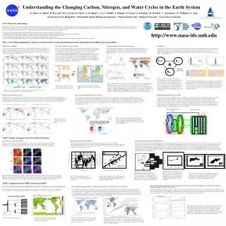
Energy, water and carbon exchange Vegetation dynamics Climate statistics Land-use transitions { t~ 30 min Atmosphere leaves Carbon gain fine roots Carbon Phenology, t~ 1 month Canopy and canopy air Fire Energy and moisture balance labile Photosynthesis Plant and soil respiration Carbon uptake and release Land-use management, t ~ 1 year Biogeography, t ~ 1 year Plant type LAI, height, roots Mortality, natural and fire t ~ 1 year Carbon allocation and growth, t ~ 1 day sapwood Soil/snow wood Human fire suppression Risk Understanding the Changing Carbon, Nitrogen, and Water Cycles in the Earth System B. Moore1, G. Hurtt1, B. Braswell1, M.G. Fearon1, B. Fekete1, S. Frolking1, C. Li1, J. Melillo2, S. Ollinger1, S. Pacala3, S. Seitzinger4, R. Stallard5, C. Vorosmarty1, W. Wollheim1, X. Xiao1 1University of New Hampshire; 2 Woods Hole Marine Biological Laboratory; 3 Princeton University; 4 Rutgers University; 5 University of Colorado Goals, Objectives, and Strategy • The goal of this research is to understand the primary biogeochemical cycles of the planet, the nature of the coupling between the biogeochemical cycles and the physical climate system, and the characteristics of the human forcing of the terrestrial-aquatic system. Our focus is on how the carbon, nitrogen, and water cycles function in natural systems and in systems perturbed by human activity and climate variability and change. These strongly interacting biogeochemical cycles play a crucial role in the future state of the Earth System. Our objectives are to address a set of important, linked scientific questions that bear directly upon global environmental change and associated policy issues. • What are the current and likely future global distributions and strengths of terrestrial sources and sinks of carbon dioxide? • Will there be strong and rapid positive or negative feedbacks in the Earth system’s response to climate forcing from increased greenhouse gas concentrations? • How will increases in N deposition and fertilization affect the long-term uptake and storage of carbon in terrestrial ecosystems? • How are humans altering the global riverine fluxes of carbon, nitrogen, and water from land to coastal oceans? • How does the intentional management of any one component of the Earth system affect other components? Are management strategies for individual components consistent with each other? http://www.nasa-ids.unh.edu Task 1. To Develop and Implement a Sequence of Integrated Terrestrial-Aquatic Biogeochemical Sub models in the GFDL Earth System Model Global Land-use Modeling Terrestrial N cycling and trace gas emissions Carbon and nitrogen dynamics in freshwater systems Fire Dynamics We have developed the first global, gridded study and set of modeling products designed to address the role of secondary forests, and include the effects of logging and shifting cultivation as well as permanent agriculture (Figure 1). This effort specifically calculated annual land-use transitions for each grid cell, and provides an essential input data layer for GCM and Earth System Models. The products are being used by our group and by other global modeling teams and IPCC estimates. Wehave developed preliminary estimates of global, gridded, annual and monthly, net nitrogen loading to land for contemporary and pre-industrial conditions to the Earth System Modeling group at GFDL; Figure 2 illustrates an example of annual nitrogen loading. We are also developing algorithms for horizontal movement of carbon and nitrogen from production sites to consumption sites (i.e., food/feed/fiber trade). We are using the DNDC model for terrestrial N-cycling simulations (Fig. 3), and also have been developing “simplified” versions of DNDC. During the past year, major progress has been made in two aspects: DNDC validation and input data acquisition. For Asia, validation focused on crop biomass/yield and fluxes of water, C and N in the agroecosystems of rice production. For Europe, validation focused on SOC dynamics and N gas emissions from forest and agricultural ecosystems. Databases of climate, soil, vegetation, and management have been or are being built up for the Monsoon Asia, North China, EU countries and Russia. We have developed datasets and models for water flux through gridded rivers networks, river corridors and engineering, sediment sources and routing, organic matter loading and processing including denitrification, and fluvial carbon sequestration sites. Predicted exports of water, DOC, DON, and DIN from upland ecosystems are being linked to an aqueous biogeochemical transport model. Our group has been actively progressing on the development and integration of fire models for global studies. Recent efforts have focused on the interpretation of satellite remote sensing of fire activity, model formulations that account for human affects on fire frequency, and a global synthesis chapter on natural disasters in the Millennium Ecosystem Assessment. These studies represent significant advances in the interpretation and modeling of fire dynamics over both temperate and tropical systems including the effects of climate, human activities (land-use etc…), and fire suppression. Figure 5. Feedback loop for carbon, fire, and risk. Arrowheads indicates a positive coupling (e.g. increased carbon-stocks leading to increased fire risk, increased fire risk leading to increased fire), open-heads indicates a negative coupling (e.g. increased fire leading to reduced carbon stocks). This system is a negative feedback loop and is is self-regulating under natural conditions. Human fire suppression can alter the system in complex ways by reducing fire, leading to carbon accumulation, and increased future fire risk. Figure 6. Burned area in the United States for the year 2000. Panel (a) compares the fire size distribution of model estimates that include fire-suppression to satellite data. The distribution of differences between model and satellite annual burned area by grid cell is shown in (b). Maps of the burned area (km2) per grid cell estimated by the model are given by (c), and reported by the GBA-2000 Project in (d). This model is being used to assess the ability to sustain carbon sinks that have resulted from human fire suppression. Figure 4. Modeling nutrient biogeochemistry of the global freshwater aquatic system using FrAMES. A) Distribution of small river, large river, lake and reservoir surface area as a function of latitude, B) Distribution of N load to aquatic systems based on terrestrial model predictions and nitrogen removal by small rivers, large rivers, lakes, and reservoirs as a function of latitude as predicted by FrAMES, and C) Predictions of within basin DIN:DIP ratio in large rivers, obtained by combining single constituent models of within basin DIP and DIN routing in FrAMES. Such patterns in nutrient stoichiometry serve as indicators of aquatic system stress and will be used to identify "hot spots" of stress or rapid change. Figure 2. Annual 1° grid cell net nitrogen loading to the land (g N m-2 y-1) for pre-industrial and contemporary conditions. Figure 3. Regional distribution of N2O and NO emissions from forest soils in Europe (from Kesik et al., 2005). Figure 1. 1° Grid cell cropland fraction, pastureland fraction, secondary land fraction, and grid cell mean age of secondary land (years) for 1800, 1900, and 2000. Planted crops and management systems Water engineering including irrigation and reservoirs Model Simplification and Integration to ESM Building on the land-use modeling described above (see Fig. 1), we have begun development of a set of products that detail the crop-types and management systems of agriculture worldwide. This information is necessary for developing model routines that accurately simulate the management activities on agricultural lands. Our approach is to build on the work of Leff et al. and to derive a global gridded product of spatial distribution functionally different crop/type management systems. Figure 7 illustrates the four GLM crop types (C3 annual, C3 perennial, C4 annual, N fixers). In order to characterize human water uptake from surface and groundwater resources, we first focused on agricultural water use, which represents 70% of all water withdrawals globally. We geospatially distributed irrigation water use data over a gridded dataset of irrigation-equipped lands based on irrigation need (grid cell PET – AET). We then compared the gridded fields of irrigation water use with WBM-generated runoff to highlight areas of potentially non-sustainable water use as shown in Figure 9. At the basin scale, we have estimated that non-sustainable irrigation water use could represent as much as 900 km3/year. We are currently perfecting an algorithm for identifying sources of irrigation water (river versus deep groundwater sources) in order to refine our estimates of non-sustainable irrigation water use. We developed a comprehensive global dynamic land model (LM3V) able to simulate carbon and vegetation dynamics, as well as to represent the exchange of water and energy between land, vegetation, and atmosphere. LM3V represents changes in vegetation communities and their biophysical and biogeochemical feedbacks to climate system. LM3V tracks carbon in vegetation and soil in response to environmental conditions, ambient concentration of CO2, natural disturbances (e.g. fire), and anthropogenic land-use changes (including deforestation, secondary forest harvesting, and agricultural cropland abandonment). For land use, it specifically draws on formulations developed for the ED model, and land-use history information developed as part of this project. LM3V is the first model in its class able to estimate the extent and effects of secondary forests in the Earth System. It has been evaluated forced with observed atmospheric data, and coupled with Geophysical Fluid Dynamics Laboratory (GFDL) atmospheric circulation model AM2. Figure 9. Comparison of gridded fields of renewable water resources with geospatially distributed irrigation withdrawals. Areas of potentially non-sustainable irrigation water use (where irrigation withdrawals are greater than renewable runoff and river flow) are highlighted in red. Figure 7. Global Cropland Distribution for the Global Land-Use and Earth System Models. TASK 2. Remote Sensing for Terrestrial Model Evaluation Land Cover and Canopy Characteristics Remote Sensing of Vegetation Productivity Remote Sensing of Canopy Nitrogen at Regional Scales The purpose of this activity is to develop and use approaches for mapping land cover distributions using data from multiple satellite observations at a variety of scales, with specific application to estimating patterns of human land use. We will particularly focus on changes that are intrinsically small in scale but spatially extensive and biogeochemically important. We used field data from eddy flux tower sites in North America and the Amazon basin to evaluate the Vegetation Photosynthesis Model (VPM). We also have developed a collaboration with Euroflux network and evaluated the VPM model with field data from 15 eddy flux tower sites in Europe, including a variety of ecosystem types (from grassland to deciduous broadleaf forests and needleleaf evergreen forests). We have examined the extent to which relationships between N concentrations and maximum photosynthesis observed at the leaf level can be extended to patterns of carbon assimilation in whole forest canopies. We have used data from five eastern U.S AmeriFlux sites to assess maximum rates of GPP in relation to landscape-level averages for canopy N concentration, derived through high spectral resolution remote sensing (Fig. 13). We've obtained a significant linear relationship between canopy GPPmax and remotely-sensed canopy N. This result has important implications for controls on terrestrial ecosystem carbon assimilation and suggests that methods for broad-scale canopy N detection are needed (Fig. 14). We have also explored relationships between vegetation N content and vegetation indices retrieved by MODIS, through spatial degradation and georegistration of high resolution canopy N estimates to coarse resolution MODIS pixels. Early results demonstrate a weak but significant relationship between foliar N predictions and both the ratio vegetation index (RVI) and the difference vegetation index (DVI), while revealing no sensitivity to vegetation N by the normalized difference vegetation index (NDVI) (Fig. 15). Figure 14. Remotely-sensed foliar N for AmeriFlux sites in eastern U.S. forest biome in relation to canopy Amax data. Relationship is independent of variation in fPAR or LAI and suggests that important spatial variation in C assimilation is driven by vegetation traits that captured by current global remote sensing instruments. Figure 13. Estimates of canopy N content for sites within the AmeriFlux network. Data have been acquired for all sites indicated and are being used to derive (a) a continental-scale relationship between canopy N and vegetation carbon assimilation capacity (GPPmax, or canopy level Amax) and (b) generalizable methods for N detection using broad-band sensors. Figure 15. Relationships between canopy N and broad-band spectral reflectance properties, as simulated using data from the AVIRIS and Hyperion Sensors. Although results indicate only a very weak relationship between foliar N and NDVI, a strong and highly significant trend was observed using the NIR band alone. Figure 10. Observed and predicted values of forest, secondary, and cleared fractional areas for the reference case in Ruropolis. Note the differences in scale associated with natural distributions of these classes within 1.1-km pixels. Grey areas are pixels with missing ETM+ or MISR data. This is close-up of an approximately 80 km2 area around the city of Ruropolis, revealing good representation of spatial patterns for the fractions, especially edge effects, and very little spatial structure in the residuals of the estimation (bottom three panels). Figure 11. The seasonal dynamics of leaf phenology clearly contributes to high rates of evapotranspiration and gross primary production in the dry season. Figure 12. Seasonal dynamics of observed evapotranspiration and predicted gross primary production from the satellite-based Vegetation Photosynthesis Model (VPM) for the CO2 eddy flux site at Tapajos, Brazil. TASK 3. Application of the GFDL Earth System Model How does the intentional management of any one component of the Earth system affect other components? Are management strategies for individual components consistent with each other? What are the current and likely future global distributions and strengths of terrestrial sources and sinks of carbon dioxide? How are humans altering the global riverine fluxes of carbon, nitrogen, and water from land to coastal oceans? Historical changes in CO2 concentrations, climate, and land-use activities all affect the terrestrial carbon cycle. We are conducting a series of modeling experiments to quantify the effects of these changes on the current patterns of terrestrial sources and sinks of carbon dioxide. We have begun use the coupled model to explore three major classes of disturbance: (1) altered hydraulics and hence altered constituent transport potential of water systems, through impoundment, irrigation and interbasin transfers; (2) assessment of land management options including continued nitrogen deposition versus mitigation strategies, varying land cover change rates, alternative industrial agricultural practices, and point source loadings; and (3) management options for carbon sequestration on land. The analysis will explore the cascade of impacts from sources through aquatic transport corridors and sink terms. We anticipate both hydraulic and biogeochemical processing controls on the linked fluxes. Within the ESM, variations in the location and strength of predicted C and N sources and sinks will be placed into a much larger context and used to study climate system feedbacks. Strategies for mitigating the increasing concentration of carbon dioxide in the atmosphere include sequestering carbon (C) in soils and vegetation of terrestrial ecosystems. Carbon and nitrogen (N) move through terrestrial ecosystems in coupled biogeochemical cycles, and increasing C stocks in soils and vegetation will have an impact on the N cycle. We conducted simulations with the DNDC biogeochemical model to evaluate the impact of different cropland management strategies on the coupled cycles of C and N, with special emphasis on C-sequestration and emission of the greenhouse gases methane (CH4) and nitrous oxide (N2O). Figure 20. Simulated soil organic C (SOC) content and annual N2O emission for conventional (solid lines) and alternative (dashed lines) management scenarios: (A) Iowa SOC; (B) Iowa N2O; (C) China SOC; (D) China N2O; (E) Bavaria SOC; (F) Bavaria N2O. Alternative management: (A&B) maize/soybean - reduced tillage, (C&D) maize/wheat - increased crop residue incorporation, and (E&F) barley - increased manure inputs. In each case the alternative management scenario led to increased SOC storage and to increased N2O emissions. Figure 16. Model experimental design. Figure 17. Model estimate of contemporary NEP accounting for historical land-use activities, CO2 increases, and climate changes. Figure 18 Global potential river network at 0.5° resolution (this includes actively draining rivers as well as those that do not flow continuously, do not drain to the oceans, and/or are covered by ice). Figure 19. We updated our reservoir database to incorporate the top 2000 reservoirs, and developed reservoir operation modules to simulate the impact of reservoir functions on discharge regime (irrigation, flood control, power generation, etc.). Figure of global sediment model showing impact of reservoir storage of sediment and the first estimates of time-varying fluxes to the world’s coastal zones.