Download
1 / 65
650 likes | 739 Views
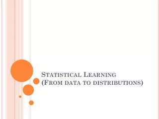
Statistical Learning (From data to distributions) . Agenda. Learning a discrete probability distribution from data Maximum likelihood estimation (MLE) Maximum a posteriori (MAP) estimation. Motivation.

E N D
Agenda • Learning a discrete probability distribution from data • Maximum likelihood estimation (MLE) • Maximum a posteriori (MAP) estimation
Motivation • Previously studied how to infer characteristics of a distribution, given a fully-specified Bayes net • This lecture: where does the specification of the Bayes net come from? • Specifically: estimating the parameters of the CPTs from fully-specified data
Learning in General • Agent has made observations (data) • Now must make sense of it (hypotheses) • Why? • Hypotheses alone may be important (e.g., in basic science) • For inference (e.g., forecasting) • To take sensible actions (decision making) • A basic component of economics, social and hard sciences, engineering, …
Machine Learning vs. Statistics • Machine Learning automated statistics • This lecture • Statistical learning (aka Bayesian learning) • Maximum likelihood (ML) learning • Maximum a posteriori (MAP) learning • Learning Bayes Nets (R&N 20.1-3) • Future lectures try to do more with even less data • Decision tree learning • Neural nets • Support vector machines • …
Putting General Principles to Practice • Note: this lecture will cover general principles of statistical learning on toy problems • Grounded in some of the most theoretically principledapproaches to learning • But the techniques are far more general • Practical applications to larger problems requires a bit of mathematical savvy and “elbow grease”
Beautiful results in math give rise to simple ideas orHow to jump through hoops in order to justify simple ideas …
Candy Example • Candy comes in 2 flavors, cherry and lime, with identical wrappers • Manufacturer makes 5 indistinguishable bags • Suppose we draw • What bag are we holding? What flavor will we draw next? h1C: 100%L: 0% h2C: 75%L: 25% h3C: 50%L: 50% h4C: 25%L: 75% h5C: 0%L: 100%
Bayesian Learning • Main idea: Compute the probability of each hypothesis, given the data • Data d: • Hypotheses: h1,…,h5 h1C: 100%L: 0% h2C: 75%L: 25% h3C: 50%L: 50% h4C: 25%L: 75% h5C: 0%L: 100%
Bayesian Learning • Main idea: Compute the probability of each hypothesis, given the data • Data d: • Hypotheses: h1,…,h5 P(hi|d) We want this… P(d|hi) But all we have is this! h1C: 100%L: 0% h2C: 75%L: 25% h3C: 50%L: 50% h4C: 25%L: 75% h5C: 0%L: 100%
Using Bayes’ Rule • P(hi|d) = a P(d|hi) P(hi) is the posterior • (Recall, 1/a = P(d) = Si P(d|hi) P(hi)) • P(d|hi) is the likelihood • P(hi) is the hypothesis prior h1C: 100%L: 0% h2C: 75%L: 25% h3C: 50%L: 50% h4C: 25%L: 75% h5C: 0%L: 100%
Likelihood and prior • Likelihood is the probability of observing the data, given the hypothesis model • Hypothesis prior is the probability of a hypothesis, before having observed any data
P(d|h1)P(h1)=0P(d|h2)P(h2)=9e-8P(d|h3)P(h3)=4e-4P(d|h4)P(h4)=0.011P(d|h5)P(h5)=0.1P(d|h1)P(h1)=0P(d|h2)P(h2)=9e-8P(d|h3)P(h3)=4e-4P(d|h4)P(h4)=0.011P(d|h5)P(h5)=0.1 P(h1|d) =0P(h2|d) =0.00P(h3|d) =0.00P(h4|d) =0.10P(h5|d) =0.90 Sum = 1/a = 0.1114 Computing the Posterior • Assume draws are independent • Let P(h1),…,P(h5) = (0.1, 0.2, 0.4, 0.2, 0.1) • d = { 10 x } P(d|h1) = 0 P(d|h2) = 0.2510 P(d|h3) = 0.510 P(d|h4) = 0.7510P(d|h5) = 110
Predicting the Next Draw H • P(X|d) = Si P(X|hi,d)P(hi|d) = Si P(X|hi)P(hi|d) D X Probability that next candy drawn is a lime P(h1|d) =0P(h2|d) =0.00P(h3|d) =0.00P(h4|d) =0.10P(h5|d) =0.90 P(X|h1) =0P(X|h2) =0.25P(X|h3) =0.5P(X|h4) =0.75P(X|h5) =1 P(X|d) = 0.975
Properties of Bayesian Learning • If exactly one hypothesis is correct, then the posterior probability of the correct hypothesis will tend toward 1 as more data is observed • The effect of the prior distribution decreases as more data is observed
Hypothesis Spaces often Intractable • To learn a probability distribution, a hypothesis would have to be a joint probability table over state variables • 2n entries => hypothesis space is 2n-1-dimensional! • 2^(2n) deterministic hypotheses6 boolean variables => over 1022 hypotheses • And what the heck would a prior be?
Learning Coin Flips • Let the unknown fraction of cherries be q (hypothesis) • Probability of drawing a cherry is q • Suppose draws are independent and identically distributed (i.i.d) • Observe that c out of N draws are cherries (data)
Learning Coin Flips • Let the unknown fraction of cherries be q (hypothesis) • Intuition: c/N might be a good hypothesis • (or it might not, depending on the draw!)
Maximum Likelihood • Likelihood of data d={d1,…,dN} given q • P(d|q) = Pj P(dj|q) = qc (1-q)N-c i.i.d assumption Gather c cherry terms together, then N-c lime terms
Maximum Likelihood • Likelihood of data d={d1,…,dN} given q • P(d|q) = qc (1-q)N-c
Maximum Likelihood • Likelihood of data d={d1,…,dN} given q • P(d|q) = qc (1-q)N-c
Maximum Likelihood • Likelihood of data d={d1,…,dN} given q • P(d|q) = qc (1-q)N-c
Maximum Likelihood • Likelihood of data d={d1,…,dN} given q • P(d|q) = qc (1-q)N-c
Maximum Likelihood • Likelihood of data d={d1,…,dN} given q • P(d|q) = qc (1-q)N-c
Maximum Likelihood • Likelihood of data d={d1,…,dN} given q • P(d|q) = qc (1-q)N-c
Maximum Likelihood • Likelihood of data d={d1,…,dN} given q • P(d|q) = qc (1-q)N-c
Maximum Likelihood • Peaks of likelihood function seem to hover around the fraction of cherries… • Sharpness indicates some notion of certainty…
Maximum Likelihood • P(d|q) be the likelihood function • The quantity argmaxq P(d|q) is known as the maximum likelihood estimate (MLE)
Maximum Likelihood • The maximum of P(d|q) is obtained at the same place that the maximum of log P(d|q) is obtained • Log is a monotonically increasing function • So the MLE is the same as maximizing log likelihood… but: • Multiplications turn into additions • We don’t have to deal with such tiny numbers
Maximum Likelihood • The maximum of P(d|q) is obtained at the same place that the maximum of log P(d|q) is obtained • Log is a monotonically increasing function • l(q) = log P(d|q) = log [ qc(1-q)N-c]
Maximum Likelihood • The maximum of P(d|q) is obtained at the same place that the maximum of log P(d|q) is obtained • Log is a monotonically increasing function • l(q) = log P(d|q) = log [ qc(1-q)N-c]= log [ qc] + log [(1-q)N-c]
Maximum Likelihood • The maximum of P(d|q) is obtained at the same place that the maximum of log P(d|q) is obtained • Log is a monotonically increasing function • l(q) = log P(d|q) = log [ qc(1-q)N-c]= log [ qc] + log [(1-q)N-c]= c log q + (N-c) log (1-q)
Maximum Likelihood • The maximum of P(d|q) is obtained at the same place that the maximum of log P(d|q) is obtained • Log is a monotonically increasing function • l(q) = log P(d|q) = c log q + (N-c) log (1-q) • At a maximum of a function, its derivative is 0 • So, dl/dq(q)= 0 at the maximum likelihood estimate
Maximum Likelihood • The maximum of P(d|q) is obtained at the same place that the maximum of log P(d|q) is obtained • Log is a monotonically increasing function • l(q) = log P(d|q) = c log q + (N-c) log (1-q) • At a maximum of a function, its derivative is 0 • So, dl/dq(q)= 0 at the maximum likelihood estimate • => 0 = c/q – (N-c)/(1-q)=> q = c/N
Other Closed-Form MLE results • Multi-valued variables: take fraction of counts for each value • Continuous Gaussian distributions: take average value as mean, standard deviation of data as standard deviation
Maximum Likelihood for BN • For any BN, the ML parameters of any CPT can be derived by the fraction of observed values in the data, conditioned on matched parent values N=1000 B: 200 E: 500 P(E) = 0.5 P(B) = 0.2 Earthquake Burglar A|E,B: 19/20A|E,B: 188/200A|E,B: 170/500A|E,B : 1/380 Alarm
Bayes Net ML Algorithm • Input: Bayes net with nodes X1,…,Xn, dataset D=(d[1],…,d[N]) • Each d[i] = (x1[i],…,xn[i]) is a sample of the full state of the world • For each node X with parents Y1,…,Yk: • For all y1Val(Y1),…, ykVal(Yk) • For all xVal(X) • Count the number of times (X=x, Y1=y1,…, Yk=yk) is observed in D. Let this bemx • Count the number of times (Y1=y1,…, Yk=yk) is observed in D. Let this bem. (note m=xmx) • Set P(x|y1,…,yk) = mx / m for all xVal(X)
Maximum Likelihood Properties • As the number of data points approaches infinity, the MLE approaches the true estimate • With little data, MLEs can vary wildly
Maximum Likelihood in candy bag example • hML = argmaxhi P(d|hi) • P(X|d) P(X|hML) P(X|hML) P(X|d) undefined h5 hML =
Back to Coin Flips • The MLE is easy to compute… but what about those small sample sizes? • Motivation • You hand me a coin from your pocket • 1 flip, turns up tails • Whats the MLE? A particularly acute problem for BN nodes with many parents!(the data fragmentation problem)
Maximum A Posteriori Estimation • Maximum a posteriori (MAP) estimation • Idea: use the hypothesis prior to get a better initial estimate than ML, without resorting to full Bayesian estimation • “Most coins I’ve seen have been fair coins, so I won’t let the first few tails sway my estimate much” • “Now that I’ve seen 100 tails in a row, I’m pretty sure it’s not a fair coin anymore”
Maximum A Posteriori • P(q|d) is the posterior probability of the hypothesis, given the data • argmaxqP(q|d) is known as the maximum a posteriori (MAP) estimate • Posterior of hypothesis q given data d={d1,…,dN} • P(q|d) = 1/a P(d|q) P(q) • Max over q doesn’t affect a • So MAP estimate is argmaxqP(d|q) P(q)
Maximum a Posteriori • hMAP = argmaxhi P(hi|d) • P(X|d) P(X|hMAP) P(X|hMAP) P(X|d) h3 h4 h5 hMAP =
Advantages of MAP and MLE over Bayesian estimation • Involves an optimization rather than a large summation • Local search techniques • For some types of distributions, there are closed-form solutions that are easily computed
Back to Coin Flips • Need some prior distribution P(q) • P(q|d) P(d|q)P(q) = qc (1-q)N-c P(q) Define, for all q, the probability that I believe in q P(q) q 0 1
MAP estimate • Could maximize qc (1-q)N-c P(q) using some optimization • Turns out for some families of P(q), the MAP estimate is easy to compute P(q) Beta distributions q 0 1
Beta Distribution • Betaa,b(q) = gqa-1 (1-q)b-1 • a, bhyperparameters > 0 • g is a normalizationconstant • a=b=1 is uniform distribution
Posterior with Beta Prior • Posterior qc (1-q)N-c P(q)= gqc+a-1 (1-q)N-c+b-1= Betaa+c,b+N-c(q) • Prediction = meanE[q]=(c+a)/(N+a+b)