Download
1 / 28
280 likes | 389 Views
Forecasting Future Annual Net Cash Flows. Definition of net cash flows Projecting future values Measurement of business risk Risk/return preferences Measurement of financial risk. Measuring Annual Net Cash Flows.

E N D
Forecasting Future Annual Net Cash Flows Definition of net cash flows Projecting future values Measurement of business risk Risk/return preferences Measurement of financial risk
Measuring Annual Net Cash Flows The value circled in red is the value which appears in the numerator of each year’s discounted annual net cash flows in the NPV capital budgeting model. Page 44
Forecasting Needs • Forecast of annual price of products from your operations • Forecast of annual cost per unit for inputs used in your operations • Forecasts any expected changes in productivity (i.e., yields)
Alternative Approaches • Market outlook information approach • Historical based approaches: • Naïve model (p. 64) • Olympic moving average (p. 65) • Time series econometric approach • Flexibility coefficient approach (p. 66) • Structural econometric approach (p. 65-67)
- 1 SD Mean + 1 SD Alternative Forecasting Approaches Non-Econometric Forecasting Approach Structural Econometric Forecasting Model Demand Supply QD = f(P, Y-T, W, ...) QS = f(P, MIC, …) QD = QS Solve for PE and QE PE QE Page 65 Page 109 Stochastic simulation of random variable (yields) generates an empirical probability distribution for price Subjective triangular probability distribition assumed annually based upon recent trends in local spot market prices
This is the probability distribution for the first year. One would expect the probability associated with the most likely scenario to decline over time, reflecting increasing uncertainty in subsequent years. Page 72
We would reject making this investment since the NPV < 0. Page 75
Ignoring risk would have led to an over evaluation of the projects NPV. Page 76
Ignoring the increasing risk would have led to the acceptance of this investment project. Page 76