Download
1 / 21
410 likes | 899 Views
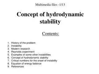
Multimedia files -1/ 13 Concept of hydrodynamic stability. Contents : History of the problem Instability Modern research Reynolds experiment Examples of some other instabilities Concept of hydrodynamic stability Critical numbers for the onset of instability Equation of energy balance

E N D
Multimedia files -1/13 Concept of hydrodynamic stability • Contents: • History of the problem • Instability • Modern research • Reynolds experiment • Examples of some other instabilities • Concept of hydrodynamic stability • Critical numbers for the onset of instability • Equation of energy balance • References
History of the problem Perhaps the first ever vortex ‘visualization’ by Leonardo da Vinci How flows become disturbed?
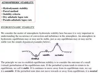
Instability Simple mechanical examples of equilibrium states: a, stable state; b, unstable state; c, neutral (indefinite) state. For certain parameters of hydrodynamic system, the hydrodynamic equations of motion with precise stationary (laminar) solutions cannot be implemented in practice: the motion is unstable. Consequently, an important subject in the theory of hydrodynamic stability is the analysis of the development of disturbances in an initially laminar flow.
Modern history of shear flow stability and transition research • Reynolds pipe flow experiment (1883) • Rayleigh’s inflection point criterion (1887) • Orr (1907) Sommerfeld (1908) viscous eq. • Heisenberg (1924) viscous channel solution • Tollmien (1929) Schlichting (1933) viscous BL solution • Schubauer & Skramstad (1948) experimental TS-wave verification • Klebanoff, Tidstrom & Sargent (1962) 3D breakdown • … Some milestones:
Reynolds experiment At certain flow parameters a laminar flow cannot remain stationary – disturbances lead to dramatic changes in it. The subject in the theory of hydrodynamic stability is the analysis of the development of the disturbances. Reynolds experiment 1883: Dye into center of pipe The flow is laminar (small velocity) Transitional flow (intermediate velocity) Developed turbulence (large velocity)
Examples of some other instabilities Benard convection at a heated plane surface Taylor vortices in flow between two rotating cylinders (Couette flow)
Illustration of flow instability (video) Click to play Video of Yu. A. Litvinenko, G.R. Grek, V.V. Kozlov and G.V. Kozlov (2010)
Concept of hydrodynamic stability • To be used in hydrodynamic applications, the definition of stability must be properly specified. Because of the complexity of the hydrodynamic equations of motion, it is obviously not possible to give a unique rational definition of the stability. In general, if at importation of certain disturbances in a flow, it returns to its initial state (speaking in the language of the theory of dynamic systems, is ‘attracted’) in time and/or space, the flow is stable to these disturbances. • Frequently in the stability problems the asymptotic (after long period) response of a system affected by a disturbance is considered. However, situations are not excluded where the disturbance at the beginning, during its establishment, experiences transient growth and only then decays. • Transient phenomena can be found in many other branches of physics, such as at the breaking of an electric circuit that can lead to a bubble break.
Electrical analogy with transient growth bulb peak voltage working voltage vout Voltage supply capacitor Transient voltage beatings A simple RC circuit. Let's consider a circuit having something other than resistors and sources. We know that vin=vR+vout. The current through the capacitor is given by and this current equals that passing through the resistor. Using vR=IR gives The input-output relation for circuits involving energy storage elements takes the form of an ordinary differential equation, which we must solve to determine what the output voltage is for a given input. Similarly, if a transient disturbance in a hydrodynamic flow becomes dangerously large during this transient growth, it can trigger the laminar–turbulent transition.
’ Disturbance source Classes of physical problems regarding the propagation of disturbances in hydrodynamic systems • The problem of initial conditions or stability in time. If the initial disturbance decays in time at each fixed point of space (or, at least, does not monotonically grow), the system is called stable to these disturbances. Otherwise, if the initial disturbance monotonically grows in time at a fixed point of space, the system is called absolutely unstable. In physiscs such systems are denoted sometimes as “generators”. In the case of the electric current there is only one independent variable (time). In hydrodynamics there are four: x,y,z,t.
Disturbance source Classes of physical problems regarding the propagation of disturbances in hydrodynamic systems • The problem of boundary conditions or amplification in space. If an external signal at the entrance to the system decays whilst propagating in it, it is said that the spatial attenuation (non-transmission of a signal) takes place. Otherwise, there is a spatial amplification, and the system is called convectively unstable. In physics such systems are called sometimes “amplifiers”.
Critical numbers for the onset of instability • The instability is defined as a state when the corresponding stability conditions are broken. In accordance with the principle of similarity first discovered experimentally by Reynolds (1883) for flow in a channel, the conditions for the appearance of the instability depend on certain dimensionless ratios of problem parameters as viscosity, density, velocity, temperature and frequency. For many simple flows, such a fundamental quantity is the Reynolds number Re=Ul/ν. Based on the definitions of stability given above, the critical Reynolds numbersseparating the regions of stable and unstable motion are defined below. • For more complex flows, such as those with curvature, other similarity parameters, e.g., the Görtler number Gö, which is a dimensionless measure of a curvature of a wall, appear. Then the same classification is applicable to them as well.
Stability of fluid motion in time • The concept of stability in time can be defined using various positive-definite norms of parameters (measures) of the disturbances. • The natural physical measure of the disturbance is usually its kinetic energy. Therefore, we give various formal definitions of the stability based on the kinetic energy of disturbance velocity u, integrated over the whole volume V covered by the hydrodynamic system • This implies either a localization of the disturbance in the volume V which is large enough for open flows (the disturbance developing only inside the volume during the observation) or the spatial periodicity of the motion for closed flows, V covering the whole range of the disturbance motion.
Definitions of stability • Asymptotic stability: A flow is (asymptotically) stable to disturbances, if where t is time. • Conditional stability: If there is a value δ > 0, such that any solution of equations of motion is stable at E(0) < δ, the solution is called conditionallystable. The value δ(the attraction radius) determines a set of initial conditions attracting to the undisturbed solution. If the disturbance energy E(0)≥δ, the disturbance grows or forms a new stable state (exchange of stability). • Global stability: If the value δ→∞, the solution is globally or unconditionallystable. • Monotonic stability: If the flow is globally stable and dE/dt ≤0 at all t > 0, the solution is monotonicallystable. As seen, each next definition imposes new restrictions on the stability.
At Re>ReE the flow loses monotonic stability; i.e. the disturbances are possible, whose energy can experience a transient growth. • At Re>ReG the flow loses global stability – it becomes conditionally stable. The sense of the conditional stability is easily seen from the simple mechanical model: the system is stable to infinitesimal disturbances, but unstable to disturbances exceeding a certain threshold value in amplitude (the ‘condition’). This is in contrast to the ‘global’ stability case. • In other words, at Re>ReG there may be initial disturbances capable, as a minimum, not to decay in time and, as a maximum, cause transition to turbulence. For such flows, where the principle of exchange of stability holds, the transition Reynolds number ReT obviously differs from ReG, i.e. stable-not-turbulent equilibrium solutions have to be taken into account.
Schematic view of the different Reynolds number regimes based on the preceding definitions • Monotonic decay (all disturbances decay) • Global stability (some disturbances may grow, but will decay, as time evolves. • Conditional stability region (only disturbances with energy more than certain value can grow without further decay) • Linear instability region (stable flow cannot exist at all) At Re>ReL the flow is linearly unstable, i.e. there is an infinitesimal disturbance which does not decrease in time. The plane Poiseuille flow and the Blasius boundary layer becomes linearly unstable at certain finite Reynolds numbers. However, there are flows such as the flow in a round pipe, which are linearly stable at any Re. [‘Linear’ means that due to the smallness of the disturbances all non-linear terms in the NS equations can be dropped.] As we will see below, global stability relates closely to the linear stability of small disturbances for the flows of our interest.
Critical Reynolds numbers for a number of wall-bounded shear flows
Equation of energy balance (Reynolds-Orr equation) • The equation of energy balance is one of the consequences of the Navier-Stokes equations for disturbances. It is obtained by multiplication of the nonlinear disturbance equation by uand integration by parts over volume V using continuity equation The procedure yields:
Equation of energy balance (Reynolds-Orr equation) In compact form it can be written as where is the symmetric deformation tensor of the mean laminar flow. As seen, the non-linear terms vanish in the equation. Due to multiplication by ui linear terms in Navier-Stokes equations correspond to quadratic terms in the equation of the energy balance. This indicates that the possible energy growth of any disturbances in incompressible Newtonian fluids is related to linear growth mechanisms.
Equation of energy balance(Reynolds-Orr equation) The first right-hand side term in the equation always negative It is known that such a maximum always exists and is positive. describes the exchange of energy with the mean flow, the second term describes the energy dissipation due to viscosity. If the exchange term is positive, the energy is extracted from the mean flow. The dissipation term is always negative. The relative value of these two terms defines whether the energy of the disturbance decays or grows. The rate of these two terms at dEV/dt = 0 forms the global stability problem for ReE, below which any disturbance monotonically decays. This can be formulated as a variational problem to search for allowablevelocities which maximize 1/ReE – the rate of two quadratic forms (the Rayleigh quotient):
References • Reynolds O. (1883) An experimental investigation of the circumstances which determine whether the motion of water shall be direct or sinuous, and of the law of resistance in parallel channels, Philos. Trans. R. Soc. Lond. A, Vol. 174, pp. 935‒982. • Lord Rayleigh (1987) On the stability, or instability, of certain fluid motions, Proc. Lond. Math. Soc., Vol. 19, pp. 67‒75. • Orr W. M'F. (1907) The stability or instability of the steady motions of a perfect liquid and of a viscous liquid. Part 2: A viscous liquid, Proc. R. Irish Acad. A, Vol. 27, pp. 69‒138. • Sommerfeld A. (1908) Ein Beitrag zur hydrodynamischen Erklärung der turbulenten Flüssigkeitsbewegungen, Atti IV Congr. Internaz. Mat., Vol. 3, pp. 116‒124. • Heisenberg W. (1924) Über Stabilität und Turbulenz von Flüssigkeitsströmen, Ann. Phys., Vol. 74, pp. 577‒627. • Tollmien W. (1929) Über die Entstehung der Turbulenz. 1. Mitteilung, Math. Phys. Klasse, Nachr. Ges. Wiss. Göttingen, 21‒44 (Translated as NACA TM 609, 1931). • Schlichting H. (1933) Zur Entstehung der Turbulenz bei der Plattenströmung, Math. Phys. Klasse, Nachr. Ges. Wiss. Göttingen, 181‒208. • Schubauer G. B. and Skramstad H. K. (1948) Laminar-boundary layer oscillations and transition on a flat plate, NACA TN‒909. • Klebanoff P. S., Tidstrom K. D., and Sargent L. M. (1962) The three-dimensional nature of boundary-layer instability, J. Fluid Mech., Vol. 12, pp. 1‒34. • Schmid P.J. and Henningson D.S. (2000) Stability and transition in shear flows, Springer, p. 1-60. • Litvinenko Yu.A., Grek G.R., Kozlov V.V. and Kozlov G.V. (2010)