Download
1 / 39
400 likes | 639 Views
Variational theory of solvation. Joachim Dzubiella Physics Department@Technical University Munich CTBP summer school 2008 „Coarse-Grained Physical Modeling of Biological Systems“. Outline . Brief intro on implicit solvation.

E N D
Variational theory of solvation Joachim Dzubiella Physics Department@Technical University Munich CTBP summer school 2008 „Coarse-Grained Physical Modeling of Biological Systems“
Outline • Brief intro on implicit solvation. • A few (explicit) systems, for which established implicit solvent models fail. • Basics of a ‚variational implicit solvent model‘ (VISM).
Motivation: biomolecular (equilibrium) processes are described by changes in the solvation free energy G: vapor or „vacuum“ Important in the modeling/description of protein assemblies, protein-ligand docking, rational drug design, etc. Quick and accurate estimates desirable.
Explicit vs. implicit solvation some protein (solute) continuum approach: (solute-solvent interface, macroscopic constants) Explicit water, e.g., molecular dynamics (MD) simulation Explicit solvent Implicit solvent
Implicit solvation: What are the dominant contributions? • ‚Hydrophobicity‘: Simple picture: water does not like to go to a (planar, nonpolar) interface; it‘s missing some of its attractive interactions; it has to rearrange. Macroscopically this gives rise to a (vapor-liquid) surface tension lv. Surface tension units: energy / surface area (A) energy penalty ~ Hydrophobic effects/interactions. A hydrophobic particle is not well solvated.
Curvature effects play an important role on small (~ 0.1-2 nm) scales: example:solvation of a hard sphere in water R Empirical expression for weak curvatures (expansion in curvature): liquid-vapor surface tension (planar interface) Symbols: MD results from Huang etal. JCP B 105, 6704 (2001) (SPC/E water, P=1bar, T=300K) Correction coefficient (historically: Tolman length)
More dominant contributions: Solute Water • Excluded volume, dispersion (van der Waals) In classical calculations: Lennard-Jones interaction • Electrostatic interactions: With a given solute charge distribution rsolve Poisson‘s equation: The energy of a charge q is Fermi repulsion van der Waals (vdW) attraction (With counterions and salt: Poisson-Boltzmann) local dielectric screening by water
Macroscopic interface thermodynamics: Free energy (grand potential) of an interfacial system: water oil R for instance an oil droplet: Note: in macroscopic considerations vdW and electrostatic attractions are all absorbed in the surface tension .
Macroscopic interface thermodynamics: Minimization of w.r.t. R yields the Young- Laplace equation: force-balance equation In general: : local mean curvature Note: example: minimal surface around two hard spheres (3-dimensional) Minimal surface equation H = 0
Established implicit solvent models Interface is defined beforehand Free energy is split into nonpolar (np) and polar (p) parts SAS MS which are evaluated separately • In general, no surface scaling on microscopic scales. • Solute-solvent interface is a prescribed input and ill-defined. • Nonpolar solvation is decoupled from electrostatics. (Many) fit-parameters depend on surface definition and solute conformations. with atomic surface area Poisson-Boltzmann/Generalized Born models
Established implicit solvent models Interface is defined beforehand Free energy is split into nonpolar (np) and polar parts SAS MS which are evaluated separately • In general, no surface scaling on microscopic scales. • Solute-solvent interface is a prescribed input and ill-defined. • Nonpolar solvation is decoupled from electrostatics. Fit-parameters depend on surface definition and solute conformations. with atomic surface area Poisson-Boltzmann/Generalized Born models Improvement by explicit consideration of vdW and volume terms Gallichio & Levy (2004), Wagoner & Baker (2006)
II. Systems, for which established implicit models conceptually fail.(selected examples)
Concave nonpolar pocket: Model for protein-ligand binding: concave pocket and one methane atom. MD simulation reveal a weakly solvated pocket and a strong hydrophobic attraction. P. Setny, JCP (2006).
Comparison to solvent accessible surface area (SASA) and molecular surface area (MSA) models: Onset of attraction is wrong by 2-4 Angstroms!
Capillary evaporation in hydrophobic confinement surface tension L~nm D T. Koishi et al., Phys. Rev. Lett. 93, 185791 (2004)
But: drastic changes to interface location and ‚nanobubble‘ stability due to strong and local water-solute attraction: • - dispersion (van der Waals) or • hydrophilic (polar) patches!
Evaporation between hydrophobic nanospheres:influence of charging. MD simulation of two hard spheres (R=1nm) in explicit water R Mean force vs distance: Catenoidal shape Surface area: JD and J.-P. Hansen, J. Chem. Phys. 121, 5514 (2004) Surface-to-surface distance
Evaporation in hydrophobic channels pore length~1nm, radius R~ 0.5nm Explicit water MD shows that a narrow hydrophobic pore can be empty of water: Nanobubble blocks ion permeation. But: pore fills when a critical electric field (E>Ec) is applied across the pore! Ions can permeate! E >Ec JD, Rosalind Allen, and J.-P. Hansen, J. Chem. Phys. 120, 5001 (2004)
Voltage-gating in biological ion channels Consistent with recent MD simulations of the MscS-channel: Narrow hydrophobic region induces evaporation. Channel ist not permeable to ions! Pore fills with application of electrostatic potential. Channel conducts! M Sotomayor et al. Ion conduction through MscS as determined by electrophysiology and simulation Biophys. J. 92, 886-902 (2007)
Evaporation in other proteins? Explicit water MD simulations of the bee venom melittin: Water in hydrophobic core. Stable nanobubble P. Liu et al., Nature 437, 159 (2005)
Established implicit solvent models Energy is split into nonpolar (np) and polar parts Interface is defined beforehand which are evaluated separately with atom surface area Poisson-Boltzmann/Generalized Born models Obviously, established models fail as interface location is predefined ! Geometric, dispersion, and electrostatic contributions have to be coupled/balanced somehow…
Variational implicit solvent model (VISM) excluded volume Define volume exclusion function: Volume Interface area Sharp kink density: Liquid water bulk density JD, J. Swanson, J. A. McCammon: J. Chem. Phys. 124, 084905 (2006); Phys. Rev. Lett. 96, 087802 (2006).
VISM free energy functional Basic idea: write the free energy G as a functional of and obtain the solute/water interface by minimization: Possible form:
Free energy functional: pressure term Energy penalty for expanding a cavity of volume V against the liquid bulk pressure P.
Free energy functional: interfacial term Separate cavity formation effects from dispersion and electrostatics Scaled particle theory or Tolman correction R liquid-vapor surface tension(planar interface) Tolman length Approximation: Symbols: MD results from Huang etal. JCP B 105, 6704 (2001) (SPC/E water, P=1bar, T=300K) with mean curvature H
Free energy functional: nonelectrostatic solute-solvent contribution accounts for excluded volumes and dispersion (van der Waals) interactions is typically modeled by the Lennard-Jones (LJ) interaction
Free energy functional: electrostatics with Variation of with respect to the electrostatic potential yields the Poisson-Boltzmann (PB) equation: solute charge density Sharp kink approximation for the position-dependent dielectric constant: dielectric constant in no-water region dielectric constant in bulk liquid
Minimization yields Gaussian curvature K=1/(R1R2) • second order partial differential equation (PDE) in terms of pressure, curvatures, dispersion, electrostatics (PB) • Generalized Laplace-Young eq. • force-per-surface-area balance equation • no analytical solution possible level-set method • ! solute is explicitly/atomistically considered in U(r) - term. • Note: electrostatics is still on a PB-level.
Example: solvation of one LJ sphere The functional reduces to a function of the radius R of the sphere: Inset: charge contribution Example: Lennard-Jones parameter = 0.2 kJ/mol and = 2.85 A.
Solvation of one uncharged LJ sphere Tolman length = fit parameter estimated from MD For SPC water:
Effective interaction between two LJ-spheres (modeling two Xe-atoms, radius~0.3nm) Water mediated interaction Best fit Tolman length: Symbols: Implicit model Red lines: Explicit water MD from D. Paschek, JCP 120, 6674 (2004) full interaction (including Xe-Xe LJ part)
Hydrophobic nanospheres (R~1nm) + charging Implicit model interface q the only fit parameter is the Tolman length Symbols: explict MD simulation Lines: theory using
Solvent evaporation between nanoplates Interfaces from Implicit model (no electrostatics here, just 2x6x6 nonpolar LJ spheres) Calculated using Effective interaction: Symbols: Implicit model Red line: Explicit water MD MD results from : T. Koishi et al., PRL 93, 185791 (2004)
Solvation of a C60 fullerene (nonpolar) Mean curvature Solvation free energy from MD: Best fit Tolman length Side note: enthalpy-entropie compensation in solvation: Solvation free energy is a difference of big numbers: Solvation entropy: Solvation enthalpy: Big problem for solvation free energy calculations!
Helical (toy) alkanes ( ~30 nonpolar LJ spheres) Mean curvature Solvation free energy from MD: Best fit Tolman length
Summary, questions, work in progress • Solute-solvent interface location at extended nonpolar surfaces sensitively depends on local geometry, dispersion, electrostatics: established implicit models fail, VISM captures the physics. but many things to do: • Numerical solution with the level-set method, marriage to PB solvers, and more benchmarking to MD simulations. • Tolman/curvature correction: testing of higher order expansion in curvature; concave/convex geometry. • Refined dielectric boundary definition to capture asymmetric solvation of cationic/anionic groups. • Interface dynamics, interface fluctuations, and coupling to molecular motions of the solute atoms. What is the interface mobility?