Download
1 / 70
700 likes | 807 Views
Last week, researchers reported on the potential benefits of coffee in preventing Parkinson's disease. But is coffee truly good for you? This text examines various studies on the effects of coffee consumption over the years, highlighting both positive and negative health outcomes associated with coffee intake. It discusses the general idea of exposure and disease in medical studies and delves into observational versus experimental study designs, with a focus on confounding variables. The advantages and limitations of observational studies, different study designs, and statistical methods for analyzing contingency tables are also explored in detail. This informative review provides insights into the complexities of studying the relationship between coffee consumption and health outcomes.

E N D
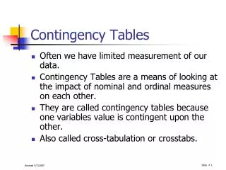
Review of observational study design and basic statistics for contingency tables
Coffee Chronicles BYMELISSA AUGUST, ANN MARIE BONARDI, VAL CASTRONOVO, MATTHEW JOE'S BLOWS Last week researchers reported that coffee might help prevent Parkinson's disease. So is the caffeine bean good for you or not? Over the years, studies haven't exactly been clear: • According to scientists, too much coffee may cause... • 1986 --phobias, --panic attacks • 1990 --heart attacks, --stress, --osteoporosis • 1991 -underweight babies, --hypertension • 1992 --higher cholesterol • 1993, 08 --miscarriages • 1994 --intensified stress • 1995 --delayed conception But scientists say coffee also may help prevent... • 1988 --asthma • 1990 --colon and rectal cancer,... • 2004—Type II Diabetes (*6 cups per day!) • 2006—alcohol-induced liver damage • 2007—skin cancer
? Exposure Disease Medical Studies The General Idea… Evaluate whether a risk factor (or preventative factor) increases (or decreases) your risk for an outcome (usually disease, death or intermediary to disease).
Observational vs. Experimental Studies Observational studies – the population is observed without any interference by the investigator Experimental studies – the investigator tries to control the environment in which the hypothesis is tested (the randomized, double-blind clinical trial is the gold standard)
Limitation of observational research: confounding • Confounding: risk factors don’t happen in isolation, except in a controlled experiment. • Example: In a case-control study of a salmonella outbreak, tomatoes were identified as the source of the infection. But the association was spurious. Tomatoes are often eaten with serrano and jalapeno peppers, which turned out to be the true source of infection. • Example: Breastfeeding has been linked to higher IQ in infants, but the association could be due to confounding by socioeconomic status. Women who breastfeed tend to be better educated and have better prenatal care, which may explain the higher IQ in their infants.
Why Observational Studies? • Cheaper • Faster • Can examine long-term effects • Hypothesis-generating • Sometimes, experimental studies are not ethical (e.g., randomizing subjects to smoke)
Possible Observational Study Designs Cross-sectional studies Cohort studies Case-control studies
Cross-Sectional (Prevalence) Studies Measure disease and exposure on a random sample of the population of interest. Are they associated? • Marginal probabilities of exposure AND disease are valid, but only measures association at a single time point.
Exposure (E) No Exposure (~E) Disease (D) a b (a+b)/T = P(D) No Disease (~D) c d (c+d)/T = P(~D) (a+c)/T = P(E) (b+d)/T = P(~E) Marginal probability of exposure Marginal probability of disease The 2x2 Table N
Example: cross-sectional study • Relationship between atherosclerosis and late-life depression (Tiemeier et al. Arch Gen Psychiatry, 2004). • Methods: Researchers measured the prevalence of coronary artery calcification (atherosclerosis) and the prevalence of depressive symptoms in a large cohort of elderly men and women in Rotterdam (n=1920).
Example: cross-sectional study P(“D”)= Prevalence of depression (sub-thresshold or depressive disorder): (20+13+12+9+11+16)/1920 = 4.2% P(“E”)= Prevalence of atherosclerosis (coronary calcification >500): (511+12+16)/1920 = 28.1%
Any depression None 28 511 53 1328 Coronary calc >500 539 1381 Coronary calc <=500 81 1839 1920 The 2x2 table: P(depression)= 81/1920 = 4.2% P(atherosclerosis) = 539/1920 = 28.1% P(depression/atherosclerosis) = 28/539 = 5.2%
Any depression None 28 511 53 1328 Coronary calc >500 539 1381 Coronary calc <=500 81 1839 1920 Difference of proportions Z-test:
Or, use relative risk (risk ratio): Any depression None 28 511 53 1328 Coronary calc >500 539 1381 Coronary calc <=500 81 1839 1920 Interpretation: those with coronary calcification are 37% more likely to have depression (not significant).
Any depression Any depression None None 539*81/1920= 22.7 28 539-22.7= 516.3 511 81-22.7= 58.3 53 1328 1381-58.3= 1322.7 Coronary calc >500 Coronary calc >500 539 539 1381 1381 Coronary calc <=500 Coronary calc <=500 81 81 1839 1839 1920 1920 Or, use chi-square test: Observed: Expected:
Chi-square test: Note: 1.77 = 1.332
Chi-square test also works for bigger contingency tables (RxC):
Chi-square test also works for bigger contingency tables (RxC):
Observed: Expected:
? Biological changes Lack of exercise Poor Eating ? Cause and effect? depression in elderly atherosclerosis
? Biological changes Lack of exercise Poor Eating ? Advancing Age Confounding? depression in elderly atherosclerosis
Cross-Sectional Studies • Advantages: • cheap and easy • generalizable • good for characteristics that (generally) don’t change like genes or gender • Disadvantages • difficult to determine cause and effect • problematic for rare diseases and exposures
2. Cohort studies: Sample on exposure status and track disease development (for rare exposures) • Marginal probabilities (and rates) of developing disease for exposure groups are valid.
Example: The Framingham Heart Study • The Framingham Heart Study was established in 1948, when 5209 residents of Framingham, Mass, aged 28 to 62 years, were enrolled in a prospective epidemiologic cohort study. • Health and lifestyle factors were measured (blood pressure, weight, exercise, etc.). • Interim cardiovascular events were ascertained from medical histories, physical examinations, ECGs, and review of interim medical record.
Example 2: Johns Hopkins Precursors Study(medical students 1948 through 1964) http://www.jhu.edu/~jhumag/0601web/study.html From the John Hopkin’s Magazine website (URL above).
Exposed Disease-free cohort Not Exposed Cohort Studies Disease Disease-free Target population Disease Disease-free TIME
Exposure (E) No Exposure (~E) Disease (D) a b No Disease (~D) c d a+c b+d risk to the exposed risk to the unexposed The Risk Ratio, or Relative Risk (RR)
Normal BP Congestive Heart Failure High Systolic BP No CHF 400 400 1500 3000 1100 2600 Hypothetical Data
Advantages/Limitations:Cohort Studies • Advantages: • Allows you to measure true rates and risks of disease for the exposed and the unexposed groups. • Temporality is correct (easier to infer cause and effect). • Can be used to study multiple outcomes. • Prevents bias in the ascertainment of exposure that may occur after a person develops a disease. • Disadvantages: • Can be lengthy and costly! 60 years for Framingham. • Loss to follow-up is a problem (especially if non-random). • Selection Bias: Participation may be associated with exposure status for some exposures
Case-Control Studies Sample on disease status and ask retrospectively about exposures (for rare diseases) • Marginal probabilities of exposure for cases and controls are valid. • Doesn’t require knowledge of the absolute risks of disease • For rare diseases, can approximate relative risk
Case-Control Studies Disease (Cases) Exposed in past Not exposed Target population Exposed No Disease (Controls) Not Exposed
Example: the AIDS epidemic in the early 1980’s • Early, case-control studies among AIDS cases and matched controls indicated that AIDS was transmitted by sexual contact or blood products. • In 1982, an early case-control study matched AIDS cases to controls and found a positive association between amyl nitrites (“poppers”) and AIDS; odds ratio of 8.6 (Marmor et al. 1982). This is an example of confounding.
Case-Control Studies in History • In 1843, Guy compared occupations of men with pulmonary consumption to those of men with other diseases (Lilienfeld and Lilienfeld 1979). • Case-control studies identified associations between lip cancer and pipe smoking (Broders 1920), breast cancer and reproductive history (Lane-Claypon 1926) and between oral cancer and pipe smoking (Lombard and Doering 1928). All rare diseases. • Case-control studies identified an association between smoking and lung cancer in the 1950’s.
Case-control example • A study of the relation between body mass index and the incidence of age-related macular degeneration (Moeini et al. Br. J. Ophthalmol, 2005). • Methods: Researchers compared 50 Iranian patients with confirmed age-related macular degeneration and 80 control subjects with respect to BMI, smoking habits, hypertension, and diabetes. The researchers were specifically interested in the relationship of BMI to age-related macular degeneration.
Case n = 50(%) Control n = 80 (%) p Value Lean BMI <20 7 (14) 6 (7.5) NS Normal 20 BMI <25 16 (32) 20 (25) NS Overweight 25 BMI <30 21 (42) 36 (45) NS Obese BMI 30 6 (12) 18 (22.5) NS NS, not significant. Results Table 2 Comparison of body mass index (BMI) in case and control groups
Overweight Normal ARMD 27 23 No ARMD 54 26 Corresponding 2x2 Table 50 80 What is the risk ratio here? Tricky: There is no risk ratio, because we cannot calculate the risk of disease!!
The odds ratio… • We cannot calculate a risk ratio from a case-control study. • BUT, we can calculate a measure called the odds ratio…
Odds vs. Risk 1:1 3:1 1:9 1:99 Note: An odds is always higher than its corresponding probability, unless the probability is 100%.
Exposure (E) No Exposure (~E) Disease (D) a b No Disease (~D) c d Odds of exposure in the cases The proportion of cases and controls are set by the investigator; therefore, they do not represent the risk (probability) of developing disease. Odds of exposure in the controls The Odds Ratio (OR) a+b=cases c+d=controls
Exposure (E) No Exposure (~E) Disease (D) a b No Disease (~D) c d Odds of exposure for the cases. Odds of disease for the exposed Odds of diseasefor the unexposed Odds of exposure for the controls The Odds Ratio (OR)
Odds of exposure in the cases Odds of exposure in the controls Bayes’ Rule Odds of disease in the exposed What we want! Odds of disease in the unexposed Proof via Bayes’ Rule (optional) =
Overweight Normal ARMD a b No ARMD c d Odds of overweight for the cases. Odds of ARMD for the overweight Odds of ARMD for the normal weight Odds of overweight for the controls The Odds Ratio (OR)
Overweight Normal ARMD 27 23 No ARMD 54 26 The Odds Ratio (OR)
Overweight Normal ARMD 27 23 No ARMD 54 26 The Odds Ratio (OR) Can be interpreted as: Overweight people have a 43% decrease in their ODDS of age-related macular degeneration. (not statistically significant here)
The odds ratio is a good approximation of the risk ratio if the disease is rare. If the disease is rare (affecting <10% of the population), then: WHY? If the disease is rare, the probability of it NOT happening is close to 1, and the odds is close to the risk. Eg:
1 1 When a disease is rare: P(~D) = 1 - P(D) 1 The rare disease assumption