Download
1 / 23
230 likes | 426 Views
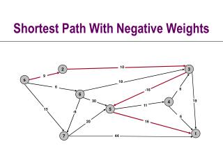
Shortest Path With Negative Weights. 2. 10. 3. 9. s. 18. 6. 6. -16. 6. 4. 19. 30. 11. 5. 15. -8. 6. 20. 16. t. 7. 44. Contents. Contents. Directed shortest path with negative weights. Negative cycle detection. application: currency exchange arbitrage

E N D
Shortest Path With Negative Weights 2 10 3 9 s 18 6 6 -16 6 4 19 30 11 5 15 -8 6 20 16 t 7 44
Contents • Contents. • Directed shortest path with negative weights. • Negative cycle detection. • application: currency exchange arbitrage • Tramp steamer problem. • application: optimal pipelining of VLSI chips
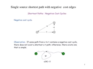
Shortest Paths with Negative Weights 3 -6 -4 7 4 5 • Negative cost cycle. • If some path from s to v contains a negative cost cycle, there does not exist a shortest s-v path; otherwise, there exists one that is simple. s v W c(W) < 0
Shortest Paths with Negative Weights • OPT(i, v) = length of shortest s-v path using at most i arcs. • Let P be such a path. • Case 1: P uses at most i-1 arcs. • Case 2: P uses exactly i arcs. • if (u, v) is last arc, then OPT selects best s-u path using at most i-1 arcs, and then uses (u, v) • Goal: compute OPT(n-1, t) and find a corresponding s-t path.
Shortest Paths with Negative Weights: Algorithm INPUT: G = (V, E), s, t n = |V| ARRAY: OPT[0..n, V] FOREACH v V OPT[0, v] = OPT[0,s] = 0 FOR i = 1 to n FOREACH v V m = OPT[i-1, v] m' = FOREACH (u, v) E m' = min (m', OPT[i-1, u] + c[u,v]) OPT[i, v] = min(m, m') RETURN OPT[n-1, t] Dynamic Programming Shortest Path
Shortest Paths: Running Time • Dynamic programming algorithm requires (mn) time and space. • Outer loop repeats n times. • Inner loop for vertex v considers indegree(v) arcs. • Finding the shortest paths. • Could maintain predecessor variables. • Alternative: compute optimal distances, consider only zero reduced cost arcs.
Shortest Paths: Detecting Negative Cycles s v C c(C) < 0 • L1: if OPT(n,v) < OPT(n-1,v) for some node v, then (any) shortest path from s to v using at most n arcs contains a cycle; moreover any such cycle has negative cost. • Proof (by contradiction). • Since OPT(n,v) < OPT(n-1,v), P has n arcs. • Let C be any directed cycle in P. • Deleting C gives us a path from s to v of fewer than n arcs C has negative cost.
Shortest Paths: Detecting Negative Cycles s 0 0 0 0 0 • L1: if OPT(n,v) < OPT(n-1,v) for some node v, then (any) shortest path from s to v using at most n arcs contains a cycle; moreover any such cycle has negative cost. • Proof (by contradiction). • Since OPT(n,v) < OPT(n-1,v), P has n arcs. • Let C be any directed cycle in P. • Deleting C gives us a path from s to v of fewer than n arcs C has negative cost. • Corollary: can detect negativecost cycle in O(mn) time. • Need to trace backthrough sub-problems. 2 18 2 6 1 -23 5 5 -11 4 -15 3
Detecting Negative Cycles: Application • Currency conversion. • Given n currencies (financial instruments) and exchange rates between pairs of currencies, is there an arbitrage opportunity? • Fastest algorithm very valuable! 8 $ F 1/7 800 3/10 4/3 2/3 2 IBM 3/50 1/10000 £ ¥ DM 170 56
Shortest Paths: Practical Improvements • Practical improvements. • If OPT(i, v) = OPT(i-1, v) for all nodes v, then OPT(i, v) are the shortest path distances. • Consequence: can stop algorithm as soon as this happens. • Maintain only one array OPT(v). • Use O(m+n) space; otherwise (mn) best case. • No need to check arcs of the form (u, v) unless OPT(u) changed in previous iteration. • Avoid unnecessary work. • Overall effect. • Still O(mn) worst case, but O(m) behavior in practice.
Shortest Paths: Practical Improvements INPUT: G = (V, E), s, t n = |V| ARRAY: OPT[V], pred[V] FOREACH v V OPT[v] = , pred[v] = OPT[s] = 0, Q = QUEUEinit(s) WHILE (Q ) u = QUEUEget() FOREACH (u, v) E IF (OPT[u] + c[u,v] < OPT[v]) OPT[v] = OPT[u] + c[u,v] pred[v] = u IF (v Q) QUEUEput(v) RETURN OPT[n-1] Bellman-Ford FIFO Shortest Path Negative cycle tweak: stop if any node enqueued n times.
Shortest Paths: State of the Art • All times below are for single source shortest path in directed graphs with no negative cycle. • O(mn) time, O(m + n) space. • Shortest path: straightforward. • Negative cycle: Bellman-Ford predecessor variables contain shortest path or negative cycle (not proved here). • O(mn1/2 log C) time if all arc costs are integers between –C and C. • Reduce to weighted bipartite matching (assignment problem). • "Cost-scaling." • Gabow-Tarjan (1989), Orlin-Ahuja (1992). • O(mn + n2 log n) undirected shortest path, no negative cycles. • Reduce to weighted non-bipartite matching. • Beyond the scope of this course.
Tramp-Steamer Problem • Tramp-steamer (min cost to time ratio) problem. • A tramp steamer travels from port to port carrying cargo. A voyage from port v to port w earn p(v,w) dollars, and requires t(v,w) days. • Captain wants a tour that achieves largest mean daily profit. 3 p = 30t = 7 p = -3t = 5 p = 12t = 3 2 1 Westward Ho (1894 – 1946) mean daily profit =
Tramp-Steamer Problem • Tramp-steamer (min cost to time ratio) problem. • Input: digraph G = (V, E), arc costs c, and arc traversal times t > 0. • Goal: find a directed cycle W that minimizes ratio • Novel application. • Minimize cycle time (maximize frequency) of logic chip on IBM processor chips by adjusting clocking schedule. • Special case. • Find a negative cost cycle.
Tramp-Steamer Problem • Linearize objective function. • Let * be value of minimum ratio cycle. • Let be a constant. • Define e = ce – te. • Case 1: there exists negative cost cycle W using lengths e . • Case 2: every directed cycle has positive cost using lengths e.
Tramp-Steamer Problem • Linearize objective function. • Let * be value of minimum ratio cycle. • Let be a constant. • Define e = ce – te. • Case 3: every directed cycle has nonnegative cost using lengths e , and there exists a zero cost cycle W*.
Tramp-Steamer Problem • Linearize objective function. • Let * be value of minimum ratio cycle. • Let be a constant. • Define e = ce – te. • Case 1: there exists negative cost cycle W using lengths e . • * < • Case 2: every directed cycle has positive cost using lengths e. • * > • Case 3: every directed cycle has nonnegative cost using lengths e , and there exists a zero cost cycle W*. • * =
Tramp-Steamer: Sequential Search Procedure Let be a known upper bound on *. REPEAT (forever) e ce – Solve shortest path problem with lengths e IF (negative cost cycle W w.r.t. e) (W) ELSE Find a zero cost cycle W* w.r.t. e. RETURN W*. Sequential Tramp Steamer • Theorem: sequential algorithm terminates. • Case 1 strictly decreases from one iteration to the next. • is the ratio of some cycle, and only finitely many cycles.
Tramp-Steamer: Binary Search Procedure W cycle left -C, right C REPEAT (forever) IF ((W) = *) RETURN W (left + right) / 2 e ce – Solve shortest path problem with lengths e IF (negative cost cycle w.r.t. e) right W negative cost cycle w.r.t. e ELSEIF (zero cost cycle W*) RETURN W*. ELSE left Binary Search Tramp Steamer left * right
Tramp-Steamer: Binary Search Procedure • Invariant: interval [left, right] and cycle W satisfy:left * (W) < right. • Proof by induction follows from cases 1-2. • Lemma. Upon termination, the algorithm returns a min ratio cycle. • Immediate from case 3. • Assumption. • All arc costs are integers between –C and C. • All arc traversal times are integers between –T and T. • Lemma. The algorithm terminates after O(log(nCT)) iterations. • Proof on next slide. • Theorem. The algorithm finds min ratio cycle in O(mn log (nCT)) time.
Tramp-Steamer: Binary Search Procedure • Lemma. The algorithm terminates after O(log(nCT)) iterations. • Initially, left = -C, right = C. • Each iteration halves the size of the interval. • Let c(W) and t(W) denote cost and traversal time of cycle W. • We show any interval of size less than 1 / (n2T2) contains at most one value from the set { c(W) / t(W) : W is a cycle }. • let W1 and W2 cycles with (W1) > (W2) • numerator of RHS is at least 1, denominator is at most n2T2 • After 1 + log2 ((2C) (n2T2)) = O(log (nCT)) iterations, at most one ratio in the interval. • Algorithm maintains cycle W and interval [left, right] s.t.left * (W) < right.
Tramp Steamer: State of the Art • Min ratio cycle. • O(mn log (nCT)). • O(n3 log2n) dense. (Megiddo, 1979) • O(n3 log n) sparse. (Megiddo, 1983) • Minimum mean cycle. • Special case when all traversal times = 1. • (mn). (Karp, 1978) • O(mn1/2 log C). (Orlin-Ahuja, 1992) • O(mn log n). (Karp-Orlin, 1981) • parametric simplex - best in practice
Optimal Pipelining of VLSI Chip • Novel application. • Minimize cycle time (maximize frequency) of logic chip on IBM processor chips by adjusting clocking schedule. • If clock signal arrive at latches simultaneously, min cycle time = 14. • Allow individual clock arrival times at latches. • Clock signal at latch: • A: 0, 10, 20, 30, . . . • B: -1, 9, 19, 29, . . . • C: 0, 10, 20, 30, . . . • D: -4, 6, 16, 26, . . . • Optimal cycle time = 10. • Max mean weight cycle = 10. A 9 B 11 7 10 14 C 5 D 6 Latch Graph