Future Climate Projections

1. Future Climate Projections

2. Lewis Richardson (1881-1953) In the 1920s, he proposed solving the weather prediction equations using numerical methods. Worked for six weeks to do a six-hour “hindcast” by hand. Proposed a wild scheme to predict the weather in real time. His scheme was totally impractical because of the lack of computing power.

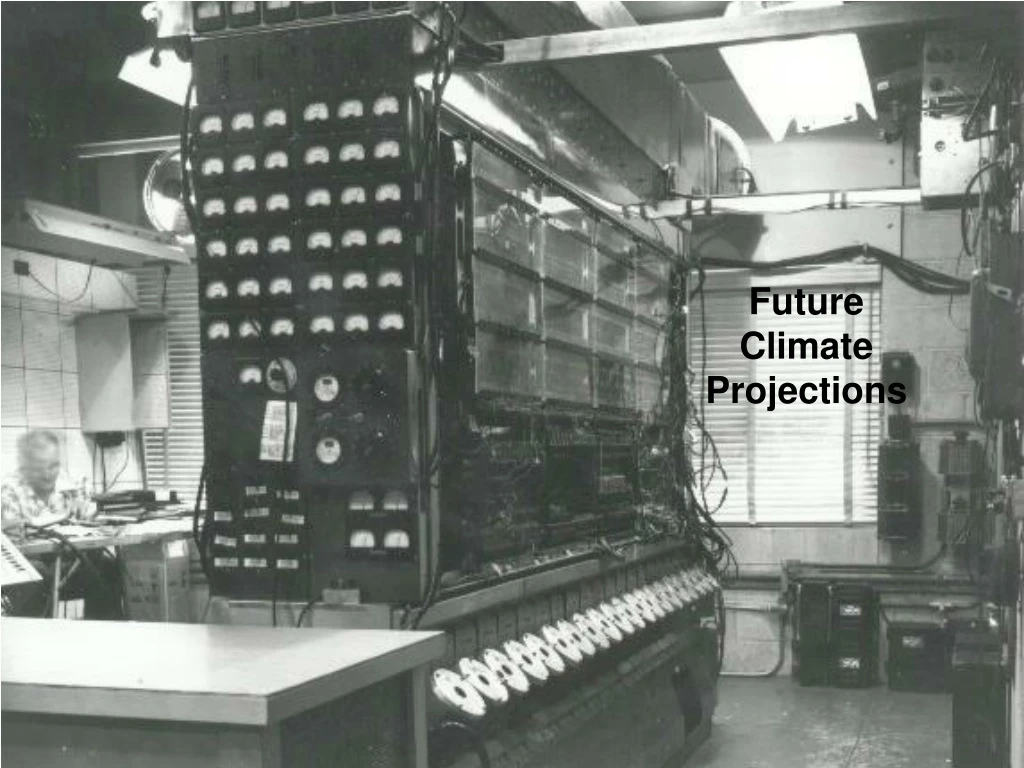
3. Over the past 50 years, there has been a remarkable increase in computing power, which has facilitated the development of numerical models to study weather and climate. We call these general circulation models (GCMs).

4. structure of a general circulation model

5. Computational grid of a general circulation model This is the typical resolution of a climate model. Note that there are many important processes for climate (such as cloud feedback), that cannot be resolved explicitly on such a coarse grid.

6. CLIMATE FEEDBACKS If the climate’s response to an increase in greenhouse gases were simply to increase its temperature to compensate for the increase in greenhouse trapping of infrared radiation, the climate change problem would be quite simple. Unfortunately, there are climate feedbacks that come into play, influencing the climate’s response. The main climate feedbacks are: (1) Water vapor feedback (2) Surface albedo feedback (3) Cloud feedback

7. WATER VAPOR FEEDBACK Water vapor feedback is thought to be a positive feedback mechanism. Water vapor feedback might amplify the climate’s equilibrium response to increasing greenhouse gases by as much as a factor of two. It acts globally. Increase in temperature Increase in water vapor in the atmosphere Enhancement of the greenhouse effect

8. SURFACE ALBEDO FEEDBACK Surface albedo feedback is thought to be a positive feedback mechanism. Its effect is strongest in mid to high latitudes, where there is significant coverage of snow and sea ice. Increase in temperature Increase in incoming sunshine Decrease in sea ice and snow cover

9. To understand how cloud feedback might work, you have to understand some facts about clouds: (1) Clouds absorb radiation in the infrared, and therefore have a greenhouse effect on the climate. If you put a cloud high in the atmosphere, it will have a stronger greenhouse effect than if you put it low in the atmosphere. (2) Clouds reflect sunshine back to space. So more clouds means less sunshine for earth. If you put a cloud high in the atmosphere, it will reflect about the same amount of sunshine as if you put a cloud low in the atmosphere.

10. Reduced greenhouse effect Which effect is stronger depends on the geographical and vertical distribution of the decrease in cloudiness Decrease in cloudiness? Increased sunshine Models predict both an increase and decrease in cloudiness, and both positive and negative cloud feedbacks. Increase in temperature CLOUD FEEDBACK Enhanced greenhouse effect Which effect is stronger depends on the geographical and vertical distribution of the increase in cloudiness Increase in cloudiness? Reduced sunshine

11. Equilibrium response of a climate model when feedbacks are removed. If the forcing associated with a doubling of CO2 is approximately 4 W/m2, what is the approximate sensitivity of each model on a global-mean basis? To calculate the climate sensitivity, we divide the response by the forcing.

12. Transient vs Equilibrium climate response Transient responserefers to the evolution of the climate system as it responds to external forcing, such as an increase in greenhouse gases. Equilibrium responserefers to the final state of the climate system after it has adjusted to the external forcing. The magnitude of the equilibrium response compared to the magnitude of the forcing is referred to as theclimate sensitivity.

13. Evolution of simulated global mean temperature when CO2 changes This shows the warming in a climate model when two scenarios of CO2 increases are imposed: one is a 1% per year increase in CO2 leading to a CO2 doubling, and the other is an increase at the same rate leading to a CO2 quadrupling. It shows that the warming continues for several centuries even when CO2 levels are stabilized, leading to significant differences between transient and equilibrium climate responses to external forcing.

14. The difference between the transient and equilibrium responses of a climate model to increasing greenhouse gases vary a great deal geographically. Which parts of the world take the longest to equilibrate to the external forcing?

15. We can also impose realistic forcing scenarios to see how well climate simulations reproduce the observed climate record. When our best guess of the observed increase in greenhouse gases and sulfate aerosols is imposed on a general circulation model, the model simulates the warming trend over the past century quite well. Note that the warming trend over the next century is projected to dwarf that of the past century. This particular model was developed at the Hadley Centre in the U.K.

16. Key Concepts Transient response Equilibrium response Climate sensitivity Water vapor feedback Surface albedo feedback Cloud feedback

17. Uncertainty about the future: This plot shows the upper and lower limits of the global mean warming over the coming century predicted by current GCM simulations. This range is due to two factors: (1) uncertainty in emissions scenarios and (2) different model sensitivities (i.e. different simulations of climate feedbacks).

18. The colors show 21st century warming taking place in response to a plausible scenario of radiative forcing. The values are averaged over all the ~20 simulations used in the most recent UN Intergovernmental Panel on Climate Change Report. The warming is calculated by subtracting temperatures at the end of the 20th century (1961-1990) from temperatures at the end of the 21st century (2071-2100).

19. The thin blue lines show the range in warming across all the models.