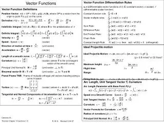
VECTOR FUNCTIONS
10. VECTOR FUNCTIONS. VECTOR FUNCTIONS. 10.3 Arc Length and Curvature. In this section, we will learn how to find: The arc length of a curve and its curvature. PLANE CURVE LENGTH.


VECTOR FUNCTIONS
E N D
Presentation Transcript
10 VECTOR FUNCTIONS
VECTOR FUNCTIONS 10.3 Arc Length and Curvature In this section, we will learn how to find: The arc length of a curve and its curvature.
PLANE CURVE LENGTH • In Section 10.2, we defined the length of a plane curve with parametric equations x = f(t), y = g(t), a≤ t ≤ bas the limit of lengths of inscribed polygons.
PLANE CURVE LENGTH Formula 1 For the case where f’ and g’ are continuous, we arrived at the following formula:
SPACE CURVE LENGTH • The length of a space curve is defined in exactly the same way.
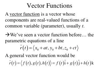
SPACE CURVE LENGTH • Suppose that the curve has the vector equation r(t) = <f(t), g(t), h(t)>, a≤ t ≤ b • Equivalently, it could have theparametric equationsx = f(t), y = g(t), z = h(t) where f’, g’ and h’ are continuous.
SPACE CURVE LENGTH Formula 2 • If the curve is traversed exactly once as t increases from a to b, then it can be shown that its length is:
ARC LENGTH Formula 3 • Notice that both the arc length formulas 1 and 2 can be put into the more compact form
ARC LENGTH • That is because: • For plane curves r(t) = f(t) i + g(t) j • For space curves r(t) = f(t) i + g(t) j + h(t) k
ARC LENGTH Example 1 • Find the length of the arc of the circular helix with vector equation • r(t) = cos ti + sin tj + tk • from the point (1, 0, 0) to the point (1, 0, 2π).
ARC LENGTH Example 1 • Since r’(t) = -sin ti + cos tj + k, we have:
ARC LENGTH Example 1 • The arc from (1, 0, 0) to (1, 0, 2π) is described by the parameter interval 0 ≤ t ≤ 2π. • So,from Formula 3, we have:
ARC LENGTH • A single curve C can be represented by more than one vector function.
ARC LENGTH Equations 4 & 5 • For instance, the twisted cubic r1(t) = <t, t 2, t 3> 1 ≤t ≤ 2 could also be represented by the function r2(u) = <eu, e2u, e3u> 0 ≤u ≤ln 2 • The connection between the parameters t and u is given by t = eu.
PARAMETRIZATION • We say that Equations 4 and 5 are parametrizationsof the curve C.
PARAMETRIZATION • If we were to use Equation 3 to compute the length of C using Equations 4 and 5, we would get the same answer. • In general, it can be shown that, when Equation 3 is used to compute arc length, the answer is independent of the parametrization that is used.
ARC LENGTH • Now, we suppose that C is a curve given by a vector function • r(t) = f(t) i + g(t) j + h(t) k a ≤t ≤b • where: • r’ is continuous. • C is traversed exactly once as t increases from a to b.
ARC LENGTH FUNCTION Equation 6 • We define its arc length functionsby:
ARC LENGTH FUNCTION • Thus, s(t) is the length of the part of C between r(a) and r(t).
ARC LENGTH FUNCTION Equation 7 • If we differentiate both sides of Equation 6 using Part 1 of the Fundamental Theorem of Calculus (FTC1), we obtain:
PARAMETRIZATION • It is often useful to parametrize a curve withrespect to arc length. • This is because arc length arises naturally from the shape of the curve and does not depend on a particular coordinate system.
PARAMETRIZATION • If a curve r(t) is already given in terms of a parameter t and s(t) is the arc length function given by Equation 6, then we may be able to solve for t as a function of s: t = t(s)
REPARAMETRIZATION • Then, the curve can be reparametrized in terms of s by substituting for t: r = r(t(s))
REPARAMETRIZATION • Thus, if s = 3 for instance, r(t(3)) is the position vector of the point 3 units of length along the curve from its starting point.
REPARAMETRIZATION Example 2 • Reparametrize the helix r(t) = cos ti + sin tj + tk with respect to arc length measured from (1, 0, 0) in the direction of increasing t.
REPARAMETRIZATION Example 2 • The initial point (1, 0, 0) corresponds to the parameter value t = 0. • From Example 1, we have: • So,
REPARAMETRIZATION Example 2 • Therefore, and the required reparametrization is obtained by substituting for t:
SMOOTH PARAMETRIZATION • A parametrization r(t) is called smoothon an interval I if: • r’ is continuous. • r’(t) ≠ 0 on I.
SMOOTH CURVE • A curve is called smoothif it has a smooth parametrization. • A smooth curve has no sharp corners or cusps. • When the tangent vector turns, it does so continuously.
SMOOTH CURVES • If C is a smooth curve defined by the vector function r, recall that the unit tangent vector T(t) is given by: • This indicates the direction of the curve.
SMOOTH CURVES • You can see that T(t) changes direction: • Very slowly when C is fairly straight. • More quickly when C bends or twists more sharply.
CURVATURE • The curvature of C at a given point is a measure of how quickly the curve changes direction at that point.
CURVATURE • Specifically, we define it to be the magnitude of the rate of change of the unit tangent vector with respect to arc length. • We use arc length so that the curvature will be independent of the parametrization.
CURVATURE—DEFINITION Definition 8 • The curvatureof a curve is: • where T is the unit tangent vector.
CURVATURE • The curvature is easier to compute if it is expressed in terms of the parameter t instead of s.
CURVATURE • So, we use the Chain Rule (Theorem 3 in Section 10.2, Formula 6) to write:
CURVATURE Equation/Formula 9 • However, ds/dt = |r’(t)| from Equation 7. • So,
CURVATURE Example 3 • Show that the curvature of a circle of radius a is 1/a. • We can take the circle to have center the origin. • Then, a parametrization is: r(t) = a cos t i + a sin t j
CURVATURE Example 3 • Therefore, r’(t) = –a sin t i + a cos t j and |r’(t)| = a • So, and
CURVATURE Example 3 • This gives |T’(t)| = 1. • So, using Equation 9, we have:
CURVATURE • The result of Example 3 shows—in accordance with our intuition—that: • Small circles have large curvature. • Large circles have small curvature.
CURVATURE • We can see directly from the definition of curvature that the curvature of a straight line is always 0—because the tangent vector is constant.
CURVATURE • Formula 9 can be used in all cases to compute the curvature. • Nevertheless, the formula given by the following theorem is often more convenient to apply.
CURVATURE Theorem 10 • The curvature of the curve given by the vector function r is:
CURVATURE Proof • T = r’/|r’| and |r’| = ds/dt. • So, we have:
CURVATURE Proof • Hence, the Product Rule (Theorem 3 in Section 10.2, Formula 3) gives:
CURVATURE Proof • Using the fact that T x T = 0 (Example 2 in Section 12.4), we have:
CURVATURE Proof • Now, |T(t)| = 1 for all t. • So,T and T’ are orthogonal by Example 4 in Section 10.2
CURVATURE Proof • Hence, by Theorem 6 in Section 12.4,
CURVATURE Proof • Thus, • and