Download
1 / 39
400 likes | 563 Views
Terra Incognita Again ;. Five zones in the mantle. Adam M. Dziewonski in cooperation with Ved Lekic and Barbara Romanowicz. KITP July 19, 2012. Convergence of 3-D models. Ritsema et al., 2011.

E N D
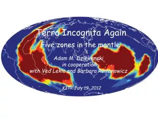
Terra Incognita Again; Five zones in the mantle Adam M. Dziewonski in cooperation with Ved Lekic and Barbara Romanowicz KITP July 19, 2012
Convergence of 3-D models Ritsema et al., 2011
Different subsets of data have to be used to recover the whole mantle structure.Models obtained using only one subset of data are shown: Left: fundamental mode Center: overtones Right: teleseismic travel times Ritsema et al., 2004
Spectral characteristics of three recent models obtained using all three subsets of data
Five zones in the mantle heterosphere Moho – 225 km upper mantle buffer zone 225-500 km transition zone 500-650 km lower mantle buffer zone 650-2400 km abyssal zone 2400 km - CMB (Dziewonski et al., 2010)
Heterosphere isotropic anisotropic
Velocity anomalies change abruptly between 200 and 300 km depth From Ritsema et al., 2004
Rapid change in the level of heterogeneity at 200 – 250 km depth: heterosphere Romanowicz (2009)
Crossing the 650 km discontinuity Model TX2008 has weak constrains in transition zone Model HMSL-S has no constraints in transition zone After Ritsema et al., 2011
Travel times of SS – SdS from 21,000 seismograms constrain topography of the 650 and 410 km discontinuities
Topography of upper mantle discontinuities Gu and Dziewonski, 2001
Correlation of TZ velocity anomalies and 660 topography High correlation of the 660km discontinuity topography with velocity perturbations in the transition zone indicates ponding of heavier (cooler) material. There is no correlation with the anomalies below 660km.
Stagnant slabs are common from Fukao et al. (2001)
LowerMantle Ritsema et al., 2011
Data and Model The dominant degree-2 signal is clearly visible in the data; the model at 2800 km depth looks very much like travel time anomalies of S-waves that bottom in the lowermost mantle.
Lower mantle “slow – fast” regionalization 5 4 3 2 1 0 How similar are regionalizations based on cluster analysis of different tomographic models? Lekic et al. (2012)
The Abyssal Layer Velocities Velocity gradient
Large scale features in different models are similar Scripps Caltech/Oxford
A puzzle: Geodynamic functions; degrees 2 & 3 only Hot spots Geoid Seismic structure Subduction 0 – 120 Ma Richards & Engerbretsen, 1992
Slabs at depth 72 km 362 km 652 km 942 km 1377 km After Lithgow-Bertelloni and Richards, 1998 2102 km j 2827 km
It does not work! Slabs and seismic velocities; Degrees 1-12 Power spectra
Slabs at depth Sum: upper mantle 72 km 362 km 652 km 942 km 1377 km After Lithgow-Bertelloni and Richards, 1998 Sum: whole mantle 2102 km j 2827 km
It works for the Upper Mantle! Comparison of seismic model S362ANI (left column) at 600 km and integrated mass anomaly for slab model L-B&R (right column). The top maps show the velocity model at 600 km and the whole-mantle integrated slab model for degrees 1-18. The bottom row shows degree-2 pattern only (note the changed color scale).
It works for the whole mantle; degrees 2 &3 only! 2800 km All degrees Degree 2 Degrees 2 & 3 Comparison of seismic model S362ANI (left column) at 2800 km and integrated mass anomaly for slab model L-B&R (right column). The top maps show the velocity model at 2800 km and the whole-mantle integrated slab model for degrees 1-18. The middle row shows degree-2 pattern only (note the changed color scale), while the third row shows the combined degree 2 and 3 pattern.
What does it mean? This means that velocity anomalies in the lowermost mantle represent a long time average of the subduction process.
Degree 2 velocity anomalies at 2800 km, the Earth’s rotation axis and TPW paths of Besse and Courtillot (2002) S362ANI SAW24B S20RTS There is less than 1 in 1,000 probability that such a configuration of degree 2 is random. If low velocities are associated with a positive gravitational effect, then the axis of the minimum moment of inertia is in the equatorial plane.
Two main points: • The characteristics of the spectrum of heterogeneity as a function of depth indicates the presence of five different regions: three in in the upper mantle and two in the lower mantle. • A very large structure at the bottom of the mantle imposes a permanent imprint on the tectonics at the surface. It determines a broad ring in which subduction can occur and regions of high hot-spot activity.
What should CIDER do? The paradigm of whole mantle convection should be modified to account of zonation of mantle heterogeneity. This will require close and constructive cooperation of geodynamicists, seismologists, mineral physicists and geochemists. CIDER has now the means to support an effort to identify the issues that need to be addressed in order to achieve substantial progress.
Principal Component Analysis (PCA) A multi-dimensional function – a 3-D velocity model, for example – may be represented by a sum of multi-dimensional functions that are orthogonal: Δv(r,θ,φ) = ∑ λi • fi (r, θ, φ) Whereλi are eigenvalues and ∫ fi • fjdV = δij The advantage of PCA is to determine the importance of different elements of the model.
Variance reduction and the radialcomponents of the largest PC’s of model S362ANI
Model obtained by using two largest PC’s compared to S362ANI (right) 69% variance reduction
Model obtained by using six largest PC’s compared to S362ANI (right) 95% variance reduction
You cannot unmix convection After 4.5 billion years after the Earth accreted, the dominant component of lateral heterogeneity in the lowermost mantle still looks like the initial model of the convection experiment
Degrees 2 & 3 tell most of the story S362ANI Degrees 2 & 3 Five model voting All degrees