Download
1 / 26
270 likes | 503 Views
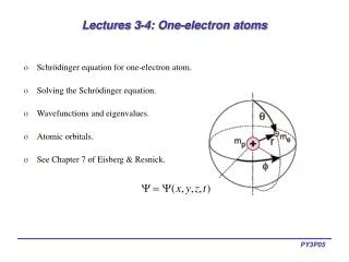
Lectures 3-4: One-electron atoms. Schrödinger equation for one-electron atom. Solving the Schrödinger equation. Wavefunctions and eigenvalues. Atomic orbitals. See Chapter 7 of Eisberg & Resnick. The Schrödinger equation. One-electron atom is simplest bound system in nature.

E N D
Lectures 3-4: One-electron atoms • Schrödinger equation for one-electron atom. • Solving the Schrödinger equation. • Wavefunctions and eigenvalues. • Atomic orbitals. • See Chapter 7 of Eisberg & Resnick. PY3P05
The Schrödinger equation • One-electron atom is simplest bound system in nature. • Consists of positive and negative particles moving in 3D Coulomb potential: • Z =1 for atomic hydrogen, Z =2 for ionized helium, etc. • Electron in orbit about proton treated using reduced mass: • Total energy of system is therefore, PY3P05
The Schrödinger equation • Using the Equivalence Principle, the classical dynamical quantities can be replaced with their associated differential operators: • Substituting, we obtain the operator equation: • Assuming electron can be described by a wavefunction of form, can write or where, is the Laplacian operator. PY3P05
The Schrödinger equation • Since V(x,y,z) does not depend on time, is a solution to the Schrödinger equation and the eigenfunction is a solution of the time-independent Schrödinger equation: • As V = V(r), convenient to use spherical polar coordinates. where • Can now use separation of variables to split the partial differential equation into a set of ordinary differential equations. (1) PY3P05
Separation of the Schrödinger equation • Assuming the eigenfunction is separable: • Using the Laplacian, and substituting (2) and (1): • Carrying out the differentiations, • Note total derivatives now used, as R is a function of r alone, etc. • Now multiply through by and taking transpose, (2) (3) PY3P05
Separation of the Schrödinger equation • As the LHS of Eqn 3does nor depend on r or and RHS does not depend on their • common value cannot depend on any of these variables. • Setting the LHS of Eqn 3 to a constant: • and RHS becomes • Both sides must equal a constant, which we choose as l(l+1): • We have now separated the time-independent Schrödinger equation into three • ordinary differential equations, which each only depend on one of (4), (5) and R(6). . (4) (5) (6) PY3P05
Summary of separation of Schrödinger equation • Express electron wavefunction as product of three functions: • As V ≠ V(t), attempt to solve time-independent Schrodinger equation. • Separate into three ordinary differential equations for and . • Eqn. 4 for () only has acceptable solutions for certain value of ml. • Using these values for mlin Eqn. 5, () only has acceptable values for certain values of l. • With these values for l in Eqn. 6, R(r) only has acceptable solutions for certain values of En. • Schrödinger equation produces three quantum numbers! PY3P05
Azimuthal solutions (()) • A particular solution of (4) is • As the einegfunctions must be single valued, i.e., => and using Euler’s formula, • This is only satisfied if ml = 0, ±1, ±2, ... • Therefore, acceptable solutions to (4) only exist when ml can only have certain integer values, i.e. it is a quantum number. • ml is called the magnetic quantum number in spectroscopy. • Called magnetic quantum number because plays role when atom interacts with magnetic fields. PY3P05
Polar solutions (()) • Making change of variables (z = rcos, Eqn.5 transformed into an associated Legendre equation: • Solutions to Eqn. 7 are of form where are associated Legendre polynomial functions. • remains finite when = 0, 1, 2, 3, ... ml = -l, -l+1, .., 0, .., l-1, l • Can write the associated Legendre functions using quantum number subscripts: 00 = 1 10 = cos1±1 = (1-cos2)1/2 • 20 = 1-3cos22±1 = (1-cos2)1/2cos • 2±2 = 1-cos2 (7) PY3P05
Spherical harmonic solutions • Customary to multiply () and () to form so called spherical harmonic functions • which can be written as: i.e., product of trigonometric and polynomial functions. • First few spherical harmonics are: Y00= 1 Y10= cos Y1±1= (1-cos2)1/2 e±i Y20= 1-3cos2 Y2±1= (1-cos2)1/2cos e±i PY3P05
Radial solutions (R( r )) • What is the ground state of hydrogen (Z=1)? Assuming that the ground state has n = 1, l = 0 Eqn. 6can be written • Taking the derivative (7) • Try solution , where A and a0are constants. Sub into Eqn. 7: • To satisfy this Eqn. for any r, both expressions in brackets must equal zero. Setting the second expression to zero => • Setting first term to zero => Same as Bohr’s results eV PY3P05
Radial solutions (R( r )) • Radial wave equation has many solutions, one for each positive integer of n. • Solutions are of the form (see Appendix N of Eisberg & Resnick): where a0is the Bohr radius. Bound-state solutions are only acceptable if where n is the principal quantum number, defined by n = l +1, l +2, l +3, … • Enonly depends on n: all l states for a given n are degenerate (i.e. have the same energy). eV PY3P05
Radial solutions (R( r )) • Gnl(Zr/a0) are called associated Laguerre polynomials, which depend on n and l. • Several resultant radial wavefunctions (Rnl( r )) for the hydrogen atom are given below PY3P05
Radial solutions (R( r )) • The radial probability function Pnl(r ), is the probability that the electron is found between r and r + dr: • Some representative radial probability functions are given at right: • Some points to note: • The r2factor makes the radial probability density vanish at the origin, even for l = 0 states. • For each state (given n and l), there are n - l - 1 nodes in the distribution. • The distribution for states with l = 0, have n maxima, which increase in amplitude with distance from origin. PY3P05
Radial solutions (R( r )) • Radial probability distributions for an electron in several of the low energy orbitals of hydrogen. • The abscissa is the radius in units of a0. s orbitals p orbitals d orbitals PY3P05
Hydrogen eigenfunctions • Eigenfunctions for the state described by the quantum numbers (n, l, ml) are therefore of form: and depend on quantum numbers: n = 1, 2, 3, … l = 0, 1, 2, …, n-1 ml = -l, -l+1, …, 0, …, l-1, l • Energy of state on dependent on n: • Usually more than one state has same energy, i.e., are degenerate. PY3P05
Born interpretation of the wavefunction • Principle of QM: the wavefunction contains all the dynamical information about the system it describes. • Born interpretationof the wavefunction: The probability (P(x,t)) of finding a particle at a position between x and x+dx is proportional to |(x,t)|2dx: P(x,t) = *(x,t) (x,t) = |(x,t)|2 • P(x,t) is the probability density. • Immediately implies that sign of wavefunction has no direct physical significance. (x,t) P(x,t) PY3P05
Born interpretation of the wavefunction • In H-atom, ground state orbital has the same sign everywhere => sign of orbital must be all positive or all negative. • Other orbitals vary in sign. Where orbital changes sign, = 0 (called a node) => probability of finding electron is zero. • Consider first excited state of hydrogen: sign of wavefunction is insignificant (P = 2 = (-)2). PY3P05
Born interpretation of the wavefunction • Next excited state of H-atom is asymmetric about origin. Wavefunction has opposite sign on opposite sides of nucleus. • The square of the wavefunction is identical on opposite sides, representing equal distribution of electron density on both side of nucleus. PY3P05
Atomic orbitals • Quantum mechanical equivalent of orbits in Bohr model. PY3P05
s orbitals • Named from “sharp” spectroscopic lines. • l = 0, ml = 0 • n,0,m = Rn,0 (r ) Y0,m (, ) • Angular solution: • Value of Y0,0is constant over sphere. • For n = 0, l = 0, ml = 0 => 1s orbital • The probability density is PY3P05
p orbitals • Named from “principal” spectroscopic lines. • l = 1, ml = -1, 0, +1 (n must therefore be >1) • n,1,m = Rn1 (r ) Y1,m (, ) • Angular solution: • A node passes through the nucleus and separates the two lobes of each orbital. • Dark/light areas denote opposite sign of the wavefunction. • Three p-orbitals denoted px, py , pz PY3P05
d orbitals • Named from “diffuse” spectroscopic lines. • l = 2, ml = -2, -1, 0, +1, +2 (n must therefore be >2) • n,2,m = Rn1 (r ) Y2,m (, ) • Angular solution: • There are five d-orbitals, denoted • m = 0 is z2. Two orbitals of m = -1 and +1 are xz and yz. Two orbitals with m = -2 and +2 are designated xy and x2-y2. PY3P05
Quantum numbers and spectroscopic notation • Angular momentum quantum number: • l = 0 (s subshell) • l = 1 (p subshell) • l = 2 (d subshell) • l = 3 (f subshell) • … • Principal quantum number: • n = 1 (K shell) • n = 2 (L shell) • n = 3 (M shell) • … • If n = 1 and l = 0 = > the state is designated 1s. n = 3, l = 2 => 3d state. • Three quantum numbers arise because time-independent Schrödinger equation contains three independent variables, one for each space coordinate. • The eigenvalues of the one-electron atom depend only on n, by the eigenfunctions depend on n, l and ml, since they are the product of Rnl(r ), lml () and ml(). • For given n, there are generally several values of l and ml => degenerate eigenfunctions. PY3P05
Orbital transitions for hydrogen • Transition between different energy levels of the hydrogenic atom must follow the following selection rules: l = ±1 m = 0, ±1 • A Grotrian diagram or a term diagram shows the allowed transitions. • The thicker the line at right, the more probable and hence more intense the transitions. • The intensity of emission/absorption lines could not be explained via Bohr model. PY3P05
Schrödinger vs. Bohr models • Schrodinger’s QM treatment had a number of advantages over semi-classical Bohr model: • Probability density orbitals do not violate the Heisenberg Uncertainty Principle. • Orbital angular momentum correctly accounted for. • Electron spin can be properly treaded. • Electron transition rates can be explained. PY3P05