Microeconomics 2
Microeconomics 2. John Hey. Office Hours of TFs. All in Alcuin SCR Daniel Howdon: Thursdays 14.00 to 15.00 James Lomas: Mondays 15.00 to 16.00 Dominic Spengler: Fridays 11.00 to 12.00. Nobel Prize Winners 2013. Eugene Fama Robert J. Shiller Lars Peter Hansen.


Microeconomics 2
E N D
Presentation Transcript
Microeconomics 2 John Hey
Office Hours of TFs • All in Alcuin SCR • Daniel Howdon: Thursdays 14.00 to 15.00 • James Lomas: Mondays 15.00 to 16.00 • Dominic Spengler: Fridays 11.00 to 12.00
Nobel Prize Winners 2013 • Eugene Fama Robert J. Shiller Lars Peter Hansen “Eugene Fama from the University of Chicago was praised for demonstrating that share prices are extremely difficult to predict in the short run, with new information quickly incorporated into prices. Robert Shiller, from Yale University, was included for his 1980s discovery that stock prices fluctuate much more than corporate dividends.” He wrote the book Irrational Exuberance. “Lars Peter Hansen, also from the University of Chicago, was awarded the prize for his development of a statistical method that was able to test theories on asset pricing.”
Nobel Prize Winners 2013 • These winners are all empirical economists who have investigated the workings of financial markets. • Their empirical work is necessarily based on theoretical models of markets. • These models are based on assumptions of rational behaviour in markets. • One crucial assumption is that of rational expectations. • This assumption ‘closes’ the models, but is empirically dubious. • At the moment, we are operating in static markets, where expectations do not play a role. • But later... • In the meantime, you should critically assess the assumptions of ‘rationality’ that we make.
Can I take stock? • Audibility? • Cannot hear • Hear too well • Perfect • Speed? • Too fast • About right • Too slow • Content? • Too difficult • About right • Too easy
What do we know? • The reservation price of a buyer is... • ...the maximum price he or she would pay. • The reservation price of a seller is ... • ...the minimum price he or she would accept.
What do we know? • The surplus of a buyer is ... • ... the area between the price paid and the demand curve. • The surplus of a seller is ... • ... the area between the price received and the supply curve. • An indifference curve is ... • ... a set of points about which the individual is indifferent.
An indifference curve and reservation prices • Beginning at the point (0,9) • Buyer • For the first unit 4 • For the second 3 • For the third 2
Reservation prices and the demand curve • [Beginning at the point (0,9)] • Buyer • For the first unit 4 • For the second 3 • For the third 2
An indifference curve and reservation prices • Starting at the point (3,0) • Seller • For the first unit 2 • For the second 3 • For the third 4
Reservation prices and the supply curve • [Starting at the point (3,3)] • Seller • For the first unit 2 • For the second 3 • For the third 4
Deduction and inference • If we know the preferences of the individual (the indifference curves or the reservation prices) and the endowment of the individual... • ...we can deduce the demand curve or the supply curve of the individual... • If instead we observe the demand and supply of the individual... • ...we can infer the preferences of the individual.
Deduction and inference The preferences of the individual (the indifference curves or the reservation prices) and the endowment Whether the individual is a buyer or a seller and either the demand or supply curve of the individual.
A Quiz • I do not like Japanese beer... • ...hence I never buy Japanese beer. • Hence my indifference curves (between money and Japanese beer) are ...? • ..... • My reservation prices (as a buyer) for Japanese beer are ....?
Chapter 4 • In Chapter 3 we have worked with a discrete good – that is, a good that can be traded in integer units. • In Chapter 4 we work with a perfectly divisible good .... which can be traded in any quantities, not only integer units. • We continue to work with a particular kind of preferences – quasi-linear ... • ... which imply indifference curves parallel in a vertical direction. • Let us go to the html file.
If you like mathematics... • m – 60/q = constant is the equation of an indifference curve – the larger the constant, the higher the indifference curve. • pq + m = 3p + 30 is the equation of the budget line. Here 3 is the endowment of the good and 30 that of money, p is the price of the good, q the quantity consumed and m the amount of money left to spend on other goods. • If we maximise the constant given the budget constraint we obtain the gross demand for the good: • q = √(60/p) • The individual begins with 3 units of the good; hence the net demand is: • q = √(60/p) – 3 • Note: this is positive if p < 60/9 = 6.66666... • is negative if p > 60/9 = 6.6666... • is zero if p = 60/9 = 6.6666....
If you like mathematics... a general proof • Take quasi-linear preferences over money m and some good q. • An indifference curve is given by k = u(q) +m (where u’(q)>0 and u’’(q) < 0 . (Why?) The higher the k the happier the individual. • We want to maximise k s.t. pq + m = pQ + M (Q,M) is endowment) • By substitution we need to maximise u(q) + PQ + M –pq w.r.t q. • The F.O.C. is u’(q) = p. This is the gross demand curve. • Original k (utility/happiness) is u(Q) + M • New k (utility/happiness) is u(q) + m = u(q) + PQ + M –pq • Increase in happiness is u(q) – u(Q) + PQ -pq • Now the area under the demand curve from Q to q is the integral from Q to q of (p = ) u’(q) minus p(q-Q). • This integral is u(q) and hence the area is • u(q) – u(Q) + PQ –pq • which is precisely the increase in happiness.
Questions for you • At what price is my demand and supply zero – that is, I am happy to stay where I am? • In this circumstance, where is the budget line in relation to the indifference curve at my endowment point?
Chapter 4 • Goodbye!