Inventory Management and Control
1.38k likes | 1.86k Views
Inventory Management and Control. Inventory Defined. Inventory is the stock of any item or resource held to meet future demand and can include: raw materials, finished products, component parts, supplies, and work-in-process. Inventory. Process stage. Number & Value. Demand Type.

Inventory Management and Control
E N D
Presentation Transcript
Inventory Defined • Inventory is the stock of any item or resource held to meet future demand and can include: raw materials, finished products, component parts, supplies, and work-in-process
Inventory Process stage Number & Value Demand Type Other Raw Material WIP Finished Goods A Items B Items C Items Maintenance Operating Independent Dependent Inventory Classifications
Independent Demand (Demand for the final end-product or demand not related to other items; demand created by external customers) Dependent Demand (Derived demand for component parts, subassemblies, raw materials, etc- used to produce final products) Independent vs. Dependent Demand Finished product Independent demand is uncertain Dependent demand is certain A B(4) C(2) D(1) E(1) E(2) B(1) E(3) Component parts
Inventory Models • Independent demand – finished goods, items that are ready to be sold • E.g. a computer • Dependent demand – components of finished products • E.g. parts that make up the computer
Types of Inventories (1 of 2) • Raw materials & purchased parts • Partially completed goods called work in progress • Finished-goods inventories (manufacturingfirms) or merchandise (retail stores)
Types of Inventories (2 of 2) • Replacement parts, tools, & supplies • Goods-in-transit to warehouses or customers
The Material Flow Cycle (2 of 2) Wait Time Queue Time Setup Time Run Time Move Time Input Output Cycle Time Run time: Job is at machine and being worked on Setup time: Job is at the work station, and the work station is being "setup." Queue time: Job is where it should be, but is not being processed because other work precedes it. Move time: The time a job spends in transit Wait time: When one process is finished, but the job is waiting to be moved to the next work area.
Performance Measures • Inventory turnover (the ratio of annual cost of goods sold to average inventory investment) • Days of inventory on hand (expected number of days of sales that can be supplied from existing inventory)
Functions of Inventory (1 of 2) • To “decouple” or separate various parts of the production process, ie. to maintain independence of operations • To meet unexpected demand & to provide high levels of customer service • To smooth production requirements by meetingseasonal or cyclical variations in demand • To protect against stock-outs
Functions of Inventory (2 of 2) 5. To provide a safeguard for variation in raw material delivery time 6. To provide a stock of goods that will provide a “selection” for customers 7. To take advantage of economic purchase-order size 8. To take advantage of quantity discounts 9. To hedge against price increases
Disadvantages of Inventory • Higher costs • Item cost (if purchased) • Holding (or carrying) cost • Difficult to control • Hides production problems • May decrease flexibility
Inventory Costs • Holding (or carrying) costs • Costs for storage, handling, insurance, etc • Setup (or production change) costs • Costs to prepare a machine or process for manufacturing an order, eg. arranging specific equipment setups, etc • Ordering costs (costs of replenishing inventory) • Costs of placing an order and receiving goods • Shortage costs • Costs incurred when demand exceeds supply
Holding (Carrying) Costs • Obsolescence • Insurance • Extra staffing • Interest • Pilferage • Damage • Warehousing • Etc.
Inventory Holding Costs(Approximate Ranges) Cost as a % of Inventory Value 6% (3 - 10%) 3% (1 - 3.5%) 3% (3 -5%) 11% (6 - 24%) 3% (2 - 5%) 26% Category Housing costs (building rent, depreciation, operating cost, taxes, insurance) Material handling costs (equipment, lease or depreciation, power, operating cost) Labor cost from extra handling Investment costs (borrowing costs, taxes, and insurance on inventory) Pilferage, scrap, and obsolescence Overall carrying cost
Ordering Costs • Supplies • Forms • Order processing • Clerical support • etc.
Setup Costs • Clean-up costs • Re-tooling costs • Adjustment costs • etc.
Shortage Costs • Backordering cost • Cost of lost sales
Inventory Control System Defined • An inventory system is the set of policies and controls that monitor levels of inventory and determinewhat levels should be maintained, when stock should be replenished and how large orders should be • Answers questions as: • When to order? • How much to order?
Objective of Inventory Control • To achieve satisfactory levels of customer service while keeping inventory costs within reasonable bounds • Improve the Level of customer service • Reduce the Costs of ordering and carrying inventory
Requirements of an Effective Inventory Management • A system to keep track of inventory • A reliable forecast of demand • Knowledge of lead times • Reasonable estimates of • Holding costs • Ordering costs • Shortage costs • A classification system
Inventory Counting (Control) Systems • Periodic System • Physical count of items made at periodic intervals; order is placed for a variable amount after fixed passage of time. • Perpetual (Continuous) Inventory System System that keeps track of removals from inventory continuously, thus monitoring current levels of each item (constant amount is ordered when inventory declines to a predetermined level)
Inventory Models • Single-Period Inventory Model • One time purchasing decision (Examples: selling t-shirts at a football game, newspapers, fresh bakery products, fresh flowers) • Seeks to balance the costs of inventory overstock and under stock • Multi-Period Inventory Models • Fixed-Order Quantity Models • Event triggered (Example: running out of stock) • Fixed-Time Period Models • Time triggered (Example: Monthly sales call by sales representative)
Single-Period Inventory Model • In a single-period model, items are received in the beginning of a period and sold during the same period. The unsold items are not carried over to the next period. • The unsold items may be a total waste, or sold at a reduced price, or returned to the producer at some price less than the original purchase price. • The revenue generated by the unsold items is called the salvage value.
3 (Newsboy Problem) • Single period model: It is used to handle ordering of perishables (fresh fruits, flowers) and other items with limited useful lives (newspapers, spare parts for specialized equipment).
Shortage cost (Cost of Understocking) • Shortage cost: generally, thiscostrepresentsunrealized profit per unit (Cu=Revenueperunit – Costperunit) • If a shortageorstockoutcostrelatesto a sparepartfor a machine, thenshortagecostreferstotheactualcost of lostproduction.
Excess cost (Cost of Over Stocking) • Excess cost (Ce): difference between purchase cost and salvage value of items left over at the end of a period. • If there is a cost associated with disposing of excess items, the salvage cost will be negative.
Single Period Model Given the costs of overestimating/underestimating demand and the probabilities of various demand sizesthe goal is to identify the order quantity or stocking level that will minimize the long-run excess (overstock)or shortage costs (understock).
Single-Period Models (Demand Distribution) • Demand may be discrete or continuous. The demand of computer, newspaper, etc. is usually an integer. Such a demand is discrete. On the other hand, the demand of gasoline is not restricted to integers. Such a demand is continuous. Often, the demand of perishable food items such as fish or meat may also be continuous. • Consider an order quantity Q • Let p = probability (demand<Q) • = probability of not selling the Qth item. • So, (1-p) = probability of selling the Qth item.
Single-Period Models (Discrete Demand) • Expected loss from the Qth item = • Expected profit from the Qth item = • So, the Qth item should be ordered if • Decision Rule (Discrete Demand): • Order maximum quantity Q such that • where p = probability (demand<Q)
Single-Period Model The service level is the probability that demand will not exceed the stocking level. The service level determines the amount of stocking level to keep.
Ce Cs Service Level Quantity So Balance point Cs Cs + Ce Service level = Optimal Stocking Level (Choosing optimum Stocking level to minimize these costs is similar to balancing a seesaw) Cs = Shortage cost per unitCe = Excess cost per unit
Service Level Another way to define ‘Service Level’ is: • proportion of cycles in which no stock-out occurs
Service Level Order Cycle Demand Stock-Outs 1 180 0 2 75 0 3 235 45 4 140 0 5 180 0 6 200 10 7 150 0 8 90 0 9 160 0 10 40 0 Total 1450 55 Since there are two cycles out of ten in which a stockout occurs, service level is 80%. This translates to a 96% fill rate. There are a total of 1,450 units demand and 55 stockouts (which means that 1,395 units of demand are satisfied).
Single Period Model (Demand is represented by a discrete distribution) • Unlike the continuous case where the optimal solution is found by determining So which makes the distribution function equal to the critical ratio cs / (cs + ce), in the discrete case, the critical ratio takes place between two values of F(So) or F(Q) • The optimal So or Qcorresponds to the higher value of F( So) or F(Q). (Note that, in the discrete case, the distribution function increases by jumps) SEE EXAMPLES 17 & 18 on page 576
Single-Period Models (Discrete Demand) Example : Demand for cookies: DemandProbability of Demand 1,800 dozen 0.05 2,000 0.10 2,200 0.20 2,400 0.30 2,600 0.20 2,800 0.10 3,000 0,05 Selling price=$0.69, cost=$0.49, salvage value=$0.29 What is the optimal number of cookies to make? c
Single-Period Models (Discrete Demand) Cs= 0.69-0.49=$0.2, Ce= 0.49-0.29=$0.2 Order maximum quantity, Q such that Demand, QProbability(demand)Probability(demand<Q), p 1,800 dozen 0.05 0.05 2,000 0.10 0.15 2,200 0.20 0.35 2,400 0.300.65 2,600 0.20 0.85 2,800 0.10 0.95 3,000 0,05 1.00
Single-Period Models (Continous Demand) • Often the demand is continuous. Even when the demand is not continuous, continuous distribution may be used because the discrete distribution may be inconvenient. • We shall discuss two distributions: Uniform distribution Normal distribution
Single-Period Models (Continuous Demand) Example 2: The J&B Card Shop sells calendars. The once-a-year order for each year’s calendar arrives in September. The calendars cost $1.50 and J&B sells them for $3 each. At the end of July, J&B reduces the calendar price to $1 and can sell all the surplus calendars at this price. How many calendars should J&B order if the September-to-July demand can be approximated by a. uniform distribution between 150 and 850
Single-Period Models (Continuous Demand) Overage cost ce = Purchase price - Salvage value =1.5-1=$0.5 Underage cost cs = Selling price - Purchase price =3-1.5=$1.5
Single-Period Models (Continuous Demand) p =0.75 Now, find the Q so that p= probability(demand<Q) =0.75 Q* = a+p(b-a) =150+0.75(850-150)=675 Probability Area Area = = 150 850 Demand * Q
Single-Period Models (Continuous Demand) Example 3: The J&B Card Shop sells calendars. The once-a-year order for each year’s calendar arrives in September. The calendars cost $1.50 and J&B sells them for $3 each. At the end of July, J&B reduces the calendar price to $1 and can sell all the surplus calendars at this price. How many calendars should J&B order if the September-to-July demand can be approximated by b. normal distribution with = 500 and =120.
Single-Period Models (Continuous Demand) Solution to Example 3: ce =$0.50, cu =$1.50 (see Example 2) p = = 0.75
Single-Period Models (Continuous Demand) Now, find the Q so that p = 0.75
Single-Period Models (Continuous Demand Q= So = mean + zσ = 500 + .68(120) = 582
Ce Cs Service Level = 75% Quantity Single Period Example 15 (pg. 574) Demand is uniformly distributed • Ce = $0.20 per unit • Cs = $0.60 per unit • Service level = Cs/(Cs+Ce) = .6/(.6+.2) • Service level = .75 • Opt. Stock.Level=S0=300+.75(500-300)= 450 liters Stockout risk = 1.00 – 0.75 = 0.25
Uniform Distribution [Continuous Dist’n] • A random variable X is uniformly distributed on the interval (a,b), U(a,b), if its pdf and cdf are: • Properties • P(x1 < X < x2) is proportional to the length of the interval [F(x2) – F(x1) = (x2-x1)/(b-a)] • E(X) = (a+b)/2V(X) = (b-a)2/12 • U(0,1) provides the means to generate random numbers, from which random variates can be generated.
Poisson Distribution [Discrete Dist’n] • Poisson distribution describes many random processes quite well and is mathematically quite simple. • where a > 0, pdf and cdf are: • E(X) = a = V(X)