Week
Week. ANOVA. Four. The ANOVA Test of Means. The F distribution is also used for testing whether two or more sample means came from the same or equal populations. This technique is called analysis of variance or ANOVA. The null and alternate hypotheses for four sample means is given as:


Week
E N D
Presentation Transcript
Week ANOVA Four
The ANOVA Test of Means The F distribution is also used for testing whether two or more sample means came from the same or equal populations. This technique is called analysis of variance or ANOVA The null and alternate hypotheses for four sample means is given as: Ho: m1 = m2 = m3 = m4 H1: m1 = m2 = m3 = m4 The ANOVA Test of Means
Underlying assumptions for ANOVA ANOVA requires the following conditions The sampled populations follow the normal distribution. The samples are independent The populations have equal standard deviations.
ANOVA Test of Means Estimate of the population variance based on the differences among the sample means Estimate of the population variance based on the variation within the samples F = If there are k populations being sampled, the numerator degrees of freedom is k – 1 Degrees of freedom for the F statistic in ANOVA If there are a total of n observations the denominator degrees of freedom is n – k.
ANOVA Test of Means ANOVA divides the Total Variation into the variation due to the treatment, Treatment Variation, and to the error component, Random Variation. In the following table, i stands for the ithobservation xG is the overall or grand mean k is the number of treatment groups
Anova Table Treatment variation Random variation Total variation
Example 1 Rosenbaum Restaurants specialize in meals for families. Katy Polsby, President, recently developed a new meat loaf dinner. Before making it a part of the regular menu she decides to test it in several of her restaurants. She would like to know if there is a difference in the mean number of dinners sold per day at the Anyor, Loris, and Lander restaurants. Use the .05 significance level.
Example 1 continued Step One: State the null hypothesis and the alternate hypothesis. Ho: mAynor = mLoris = mLandis H1: mAynor = mLoris = mLandis Step Two: Select the level of significance. This is given in the problem statement as .05. Step Three: Determine the test statistic. The test statistic follows the F distribution.
Example 1 continued Step Four: Formulate the decision rule. The numerator degrees of freedom, k-1, equal 3-1 or 2. The denominator degrees of freedom, n-k, equal 13-3 or 10. The value of F at 2 and 10 degrees of freedom is 4.10. Thus, H0 is rejected if F>4.10 or p< a of .05. Step Five: Select the sample, perform the calculations, and make a decision. Using the data provided, the ANOVA calculations follow.
Computation of SSE i k SS(Xi.k-Xk)2
Example 1 continued Computation of TSS Computation of TSSi S(Xi-XG)2
Example 1 continued Computation of SST Computation of SST k Snk(Xk-XG)2 Shortcut: SST = TSS – SSE = 86 – 9.75 = 76.25
The p(F> 39.103) is .000018. At least two of the treatment means are not the same. Since an F of 39.103 > the critical F of 4.10, the p of .000018 < a of .05, the decision is to reject the null hypothesis and conclude that The mean number of meals sold at the three locations is not the same. The ANOVA tables on the next two slides are from the Minitab and EXCEL systems. Example 1 continued
Analysis of Variance Source DF SS MS F P Factor 2 76.250 38.125 39.10 0.000 Error 10 9.750 0.975 Total 12 86.000 Individual 95% CIs For Mean Based on Pooled StDev Level N Mean StDev ---------+---------+---------+------- Aynor 4 12.750 0.957 (---*---) Loris 4 11.500 1.291 (---*---) Lander 5 17.000 0.707 (---*---) ---------+---------+---------+------- Pooled StDev = 0.987 12.5 15.0 17.5 Example 1 continued