Cochlear Model Stability & Linear Fractional Transformations
Investigating cochlear model stability using linear fractional transformations with interconnections to assess system robustness and tolerances for stability. The study utilizes the LFT modeling framework to analyze the impact of inhomogeneities and uncertainties in the cochlear system, exploring the bounds of parametric perturbations and feedback gains for guaranteed stability.

Cochlear Model Stability & Linear Fractional Transformations
E N D
Presentation Transcript
vector of active pressures p1 p0 u1 T1 vector of transformedstereocilia deflections pa,1 z1 p1 p2 p2 p1 u2 T2 pa,2 p0 z2 G3 p3 p2 p4 p3 p2 p3 u3 T3 pa,3 z3 p4 Cochlear Model The 1-D longwave model was assumed, with micromechanics shown in Fig 1. p3 p3 p2 pN-1 p1 pN=0 sound source, middle ear, and stapes helico-trema Fig 1: The discrete model of the cochlea including the details of the micromechanical model shown for element number 3. The micro-mechanical model is based on a Neely and Kim con-figuration, with details given in Elliott et al. (2007). For element i, pi(or p) is the BM pressure difference; wi,(or wBM)is the BM displacement; pa,i (or pa) is the active pressure; and wTM is a transformed tectorial membrane displacement. s2 r2 r3 s3 pa pd p s1 r1 Results: Instability due to parametric perturbations Inhomogeneities along the BM can be represented as a vector of perturbations, = [1 2 ... N]. The block in Fig. 4 is then the matrix, N = [ I + diag() ] where is a constant determining the overall gain. The question is, if we allow all the i’s to vary arbitrarily, within bounds of ±MAX then what is the value of MAX that ensures stability? The exact solution to this problem is not trivial (it is NP-hard, which is practice means that computational time becomes prohibitive for large values of N). However, a partial solution can be obtained using by a technique called -analysis. LFT modelling: Block diagram of single element To apply LFT methods to the cochlear model, first the second-order finite-difference equations representing the fluid-BM coupling, and BM micromechanical dynamics are implemented as a block diagram for a single element, as in Fig. 2. (Prempain E & Lineton B. 2009) This is a structured singular value test (Packard and Doyle, 1993; Zhou et al., 1995), which can be applied to a matrix that is readily determined from the formulation in Fig. 4, and which yields bounds on the value of MAX. The result for the model of Elliott et al. (2007) is shown in Fig. 5, with =0.8. Thus, from the peak in the curve of 12.5%, it reveals that a variation of up to 8.5% in feedback gain at each element can be tolerated, with guaranteed system stability. GN p0 Fig. 5: Bounds on 1/MAX. _ + + + + + Fig 2: Block diagram of the ith element, with inputs pi-1, pi+1 and pa,i, and outputs, pi, ui, and zi . The matrices Ai, Bi, Ci, and Fi contain the structural parameters defining the micromechanics, and is a constant arising in the finite difference approximation to the governing wave-equation. The relationship of pa,ito ui remains unspecified at this “open-loop” stage in the formulation. state-vector of ith element active outer hair cell pressure transformedstereocilia deflection Investigating cochlear model stability using linear fractional transformations Ben Lineton1 and Emmanuel Prempain2 1ISVR, University of Southampton, UK; 2Department of Engineering, University of Leicester, UK • Aims • To use the linear fractional transformations (LFT) modelling framework to reconstruct an existing state-space model of the cochlea in terms of a stable linear system with interconnections to an operator containing any desired parametric uncertainties (or perturbations such as inhomogeneities) and any non-linearities. • To use this framework to answer the question: How large can the inhomogeneities be before the model becomes unstable, thus generating SOAEs? This question is non-trivial because the inhomogeneities take the form of different perturbations in the BM parameters at each point along the BM, all of which interact with each other. LFT modelling: Interconnecting elements The block diagram in Fig. 2 can be written as a single block, Ti. The blocks for all the elements can then be connected together as shown in Fig. 3, for the first three blocks. Continuing the interconnection of all N elements, and applying the boundary conditions at the stapes and helicotrema, leads to the full cochlear model in LFT form. Motivation for using LFT LFT is an analytical method used in the field of robust control system design, which has many uses, such as investigating the effect of parametric uncertainty on a system’s stability and performance, or the effect of introducing non-linearities (Zhou et al., 1995). It is also particularly easy to implement such models using packages such as SIMULINK . Fig 3: Left: Interconnection of the first three elemental blocks. Ti is a 6 x 3 matrix representing Fig 2 in the Laplace domain. Right: The three interconnected elements are combined to form, G3 (expressed as a 16 x 5 matrix), together with the feedback block, 3. The transformation labelled “LFT” is the so-called Redheffer star-product (Zhou et al., 1995), which allows the calculation of the Gi s from the Tis recursively. G0 is a 2 x 2 matrix depending on the basal boundary condition. Thus the LFT formulation expresses the model as a stable linear system, GN, with a feedback connection to the system, N, which contains all the parametric uncertainty (and any non-linearity, if desired). In the following analysis, this formulation has been used to find the bounds on the size of the inhomogeneities within which the linear model is guaranteed to remain stable. Fig 4: Full model in LFT form. % • Summary and conclusions • LFT methods can be applied to existing discrete cochlear models, giving a model formulation in terms of a stable linear system connected via a closed-loop feedback path to a block containing any desired non-linearities and parametric uncertainties. • The LFT formulation admits various analyses, such as a test of the degree of parametric uncertainty that may lead to system instability. • An example described here yields the bounds on the variation in the BM gain that guarantee model stability. This can be interpreted as the bounds on the size of BM inhomogeneities below which SOAEs will not be generated (irrespective of the actual pattern of inhomogeneities). References Elliott SJ, Ku EM, & Lineton B. 2007. A state space model for cochlear mechanics. J Acoust Soc Am. 122, 2759-71. Packard A & Doyle JC. 1993. The complex structured singular value. Automatica, 29, 71-109. Prempain E & Lineton B. 2009. Cochlear Modelling using a Linear Fractional Transformation Approach, ICCAS-SICE, Aug. 18-21, Fukuoka, Japan, August 2009. Zhou K, Doyle J, & Glover K. 1995. Robust and Optimal Control. New Jersey, Prentice-Hall, pp. 247-69. Acknowledgements The study is part of the project entitled “Modelling and Measurements of Cochlear Gain Control” funded by the EPSRC within the Collaborating for Success in System Biology Discipline Hopping scheme.