Sorting: A Deeper Look
16. Sorting: A Deeper Look. OBJECTIVES. In this chapter you will learn: To determine the efficiency of searching and sorting algorithms and express it in “ Big O ” notation. To sort an array using the selection sort algorithm. To sort an array using the insertion sort algorithm.

Sorting: A Deeper Look
E N D
Presentation Transcript
16 • Sorting:A Deeper Look
OBJECTIVES In this chapter you will learn: • To determine the efficiency of searching and sorting algorithms and express it in “Big O” notation. • To sort an array using the selection sort algorithm. • To sort an array using the insertion sort algorithm. • To sort an array using the recursive merge sort algorithm. • To explore additional recursivesorts, including quicksort and a recursive version of selection sort. • To explore the bucket sort, which achieves very high performance, but by using considerably more memory than the other sorts we have studied—an example of the so-called “space–time trade-off.”
Recall: 6.6 Sorting Arrays • Sorting data • Important computing application • Virtually every organization must sort some data • Bubble sort (sinking sort) • Several passes through the array • Successive pairs of elements are compared • If increasing order (or identical ), no change • If decreasing order, elements exchanged • Repeat • Example: • original: 3 4 2 6 7 • pass 1: 3 2 4 6 7 • pass 2: 2 3 4 6 7 • Small elements "bubble" to the top
16.1 Introduction • Sorting data • Place data in order • Typically ascending or descending • Based on one or more sort keys • Algorithms • Insertion sort • Selection sort • Merge sort • More efficient, but more complex
16.1 Introduction (Cont.) • Big O notation • Estimates worst-case runtime for an algorithm • How hard an algorithm must work to solve a problem
16.2 Big O Notation • Big O notation • Measures runtime growth of an algorithm relative to number of items processed • Highlights dominant terms • Ignores terms that become unimportant as n grows • Ignores constant factors
16.2 Big O Notation (Cont.) • Constant runtime • Number of operations performed by algorithm is constant • Does not grow as number of items increases • Represented in Big O notation as O(1) • Pronounced “on the order of 1” or “order 1” • Example • Test if the first element of an n-array is equal to the second element • Always takes one comparison, no matter how large the array
16.2 Big O Notation (Cont.) • Linear runtime • Number of operations performed by algorithm grows linearly with number of items • Represented in Big O notation as O(n) • Pronounced “on the order ofn” or “order n” • Example • Test if the first element of an n-array is equal to any other element • Takes n - 1 comparisons • n term dominates, -1 is ignored
16.2 Big O Notation (Cont.) • Quadratic runtime • Number of operations performed by algorithm grows as the square of the number of items • Represented in Big O notation as O(n2) • Pronounced “on the order of n2” or “order n2” • Example • Test if any element of an n-array is equal to any other element • Takes n2/2–n/2 comparisons • n2 term dominates, constant 1/2 is ignored, -n/2 is ignored
Fig. 16.5| Approximate number of comparisons for common Big O notations.
16.3 Selection Sort • Selection sort • At ith iteration • Swaps the ith smallest element with element i • After ith iteration • Smallest i elements are sorted in increasing order in first i positions • Requires a total of (n2–n)/2 comparisons • Iterates n - 1 times • In ith iteration, locating ith smallest element requires n–i comparisons • Has Big O of O(n2)
Outline fig16_01.c (1 of 4 )
Outline fig16_01.c (2 of 4 ) Store the index of the smallest element in the remaining array Iterate through the whole array length– 1 times Initializes the index of the smallest element to the current item Determine the index of the remaining smallest element Place the smallest remaining element in the next spot
Outline Swap two elements fig16_01.c (3 of 4 )
Outline fig16_01.c (4 of 4 )
16.4 Insertion Sort • Insertion sort • At ith iteration • Insert (i + 1)th element into correct position with respect to first i elements • After ith iteration • First i elements are sorted • Requires a worst-case of n2 inner-loop iterations • Outer loop iterates n - 1 times • Inner loop requires n– 1iterations in worst case • For determining Big O, nested statements mean multiply the number of iterations • Has Big O of O(n2)
Outline fig16_02.c (1 of 4 )
Outline fig16_02.c (2 of 4 ) Holds the element to be inserted while the order elements are moved Iterate through length - 1 items in the array Keep track of where to insert the element Stores the value of the element that will be inserted in the sorted portion of the array Loop to locate the correct position to insert the element Moves an element to the right and decrement the position at which to insert the next element
Outline Inserts the element in place fig16_02.c (3 of 4 )
Outline fig16_02.c (4 of 4 )
16.5 Merge Sort • Merge sort • Sorts array by • Splitting it into two equal-size subarrays • If array size is odd, one subarray will be one element larger than the other • Sorting each subarray • Merging them into one larger, sorted array • Repeatedly compare smallest elements in the two subarrays • The smaller element is removed and placed into the larger, combined array
16.5 Merge Sort (Cont.) • Our recursive implementation • Base case • An array with one element is already sorted • Recursion step • Split the array (of ≥ 2 elements) into two equal halves • If array size is odd, one subarray will be one element larger than the other • Recursively sort each subarray • Merge them into one larger, sorted array
16.5 Merge Sort (Cont.) • Merge sort (Cont.) • Sample merging step • Smaller, sorted arrays • A: 4 10 34 56 77 • B: 5 30 51 52 93 • Compare smallest element in A to smallest element in B • 4 (A) is less than 5 (B) • 4 becomes first element in merged array • 5 (B) is less than 10 (A) • 5 becomes second element in merged array • 10 (A) is less than 30 (B) • 10 becomes third element in merged array • Etc.
Outline fig16_03.c (1 of 8 )
Outline fig16_03.c (2 of 8 ) Call function sortSubArray with 0 and length – 1 as the beginning and ending indices Test the base case Split the array in two
Outline fig16_03.c (3 of 8 ) Recursively call function sortSubArray on the two subarrays Combine the two sorted arrays into one larger, sorted array
Outline Loop until the end of either subarray is reached fig16_03.c (4 of 8 ) Test which element at the beginning of the arrays is smaller Place the smaller element in the combined array Fill the combined array with the remaining elements of the right array or… …else fill the combined array with the remaining elements of the left array Copy the combined array into the original array
Outline fig16_03.c (5 of 8 )
Outline fig16_03.c (6 of 8 )
Outline fig16_03.c (7 of 8 )
Outline fig16_03.c (8 of 8 )
16.5 Merge Sort (Cont.) • Efficiency of merge sort • n log n runtime • arrays means log 2 n levels to reach base case • Doubling size of array requires one more level • Quadrupling size of array requires two more levels • O(n) comparisons are required at each level • Calling sortSubArray with a size-n array results in • Two sortSubArray calls with size-n/2 subarrays • A merge operation with n– 1 (order n) comparisons • So, always order n total comparisons at each level • Represented in Big O notation as O(n logn) • Pronounced “on the order of n log n” or “order n log n”
Unsorted Single-subscripted Array of Positive Integers • n: the number of values in the array • Method: • Using a double-subscripted array of integers • With rows subscripted from 0 to 9 and • Columns subscripted from 0 to n-1 Bucket Sort (Exercise 16.6)
The bucket sort is guaranteed to have all the values properly sorted after processing the leftmost digit of the largest number. The bucket sort knows it is done when all the values are copied into row zero of the double-subscripted array. Bucket Sort: Algorithm
29 25 3 49 9 37 21 43 Bucket Sort: Algorithm
Better Performance • More Memory • Bucket sort but requires much larger storage capacity • Bubble sort requires only one additional memory location for the type of data being sorted Bucket Sort vs. Bubble Sort
Recursive Sorting Quicksort
How to determine the final position of the first element of each subarray? Quicksort