Download
1 / 68
700 likes | 920 Views
A GENETIC ALGORITHM TO SOLVE SOME SPECIAL FUNCTIONS. BY EMMANUEL SARKODIE ADABOR SUPERVISED BY MR. J. ACKORA-PRAH. OUTLINE. BACKGROUND STATEMENT OF PROBLEM OBJECTIVE METHODOLOGY APPLICATIONS TO SPECIAL FUNCTIONS CONCLUSION RECOMMENDATIONS. BACKGROUND.

E N D
A GENETIC ALGORITHM TO SOLVE SOME SPECIAL FUNCTIONS BY EMMANUEL SARKODIE ADABOR SUPERVISED BY MR. J. ACKORA-PRAH
OUTLINE BACKGROUND STATEMENT OF PROBLEM OBJECTIVE METHODOLOGY APPLICATIONS TO SPECIAL FUNCTIONS CONCLUSION RECOMMENDATIONS
BACKGROUND Darwin’s principle of survival of the fittest was used as a starting point in introducing evolutionary computation (EC). EC has four stages of development namely; Genetic algorithms (Holland, 1975) Genetic programming (Koza, 1992, 1994) Evolutionary strategies (Rocheuberg,1973)
BACKROUND (CONT.) Evolutionary programming (Forgel et al.1966) The following principles in Darwin’s principle of the survival of the fittest inspired the genetic algorithm: Species live in a competitive world. Survival depends on the fitness competition and offspring who are stronger than or equally as strong as their parents.
BACKROUND (CONT.) 3. The offspring genetically take the characteristics of their parents 4. The offspring are however unique and there is probability of slight variations in some of their genes. 5. In the competitive environment less fit individuals die off and may not become parents for breeding.
PROBLEM STATEMENT Evolutionary concepts are of recent interest since some methods may not lead to the global optimum. There is therefore the need to find an algorithm that exhausts the entire search space for the global optima of problems
OBJECTIVE A GA is applied to solve Rosenbrock’s function, Rastrigin’s function and the Schwefel’s function to test its ability to search for global optima of complex, multivariable and multimodal problems.
METHODOLOGY A GA is a search technique used in computing to find approximate solutions to optimization and search problems through application of the principles of evolutionary biology. Terms associated with GA’s are defined as follows: An individual is a solution of optimization problem
DEFINITION (CONT’D) A population is set of solutions that form the domain search space. A generation is a set of solutions taken from the population and generated at an instant of time or iteration. Selection is the operation of selecting parents from the generation to produce offspring. Crossover is the process of taking two parents and producing from them a child.
DEFINITION (CONT’D) Mutation is random operation whereby the allele of the gene in a chromosome of the offspring is changed by a probability. Recombination is the operation whereby elements of the offspring form an intermediate generation and less fit chromosomes are taken from the generation Chromosomes represent the data structure of solutions.
OVERVIEW OF GA Create initial population Evaluate the fitness of each individual Evaluation Select parent based on fitness Selection Create new population Recombination
EXAMPLE TO ILLUSTRATE OPERATORS AND OPERATIONS IN GA Max f (x) = x² for x = 0,1, … 31; Encoding: representing individual genes. Encoding may be Binary, Octal, Hexadecimal or Permutation encodings Binary encoding is used to solve the example
Solution Using a five bit (binary integer) unsigned integer, numbers between 0(00000) and 31(11111) can be obtained. Population of size 4 is randomly initialized. Selection: choosing two parents from the population for crossing. Selection Methods include Roulette Wheel, Random, Rank, Tournament and Elitist selections
ROULETTE WHEEL Roulette wheel selection is used. A roulette wheel is constructed with the cumulative and relative fitness ( f ) of chromosomes. Let i denote ith chromosome. The relative fitness of each chromosome is
ROULETTE WHEEL (CONT’D) The expected count is calculated by Where n is population size and i is the i-th chromosome
Roulette Wheel is formed as s4 13.26% s3 s1 2.16% 12.47% 54.11% s2
Crossover The various crossover techniques include single point, two point, multipoint and uniform crossovers. In a single point crossover, the parents are cut at corresponding points and the sections after the cut are exchanged.
Crossover cont’d Parent 1 0 1 1 0 0 Parent 2 1 1 0 0 1 Offspring 1 0 1 1 0 1 Offspring 2 1 1 0 0 0 Similar action is performed for the next strings resulting
Mutation Mutation prevents the algorithm to be trapped in a local minimum by maintaining diversity in population Different forms of Mutation include flipping, interchanging and reversing. Flipping is used.
Solution cont’d Replacements are made by comparing fitness values. The example was solved with crossover and mutation probabilities 1.0 and 0.001. The procedure showed an improvement on maximum fitness from 625 to 841 in just one generation.
Convergence Criteria Maximum generation Elapsed time No change in fitness Stall generations Stall time limit
APPLICATION OF GA TO SPECIAL FUNCTIONS The GA is used to solve Rosenbrock’s function, Rastrigin’s function and Schwefel’s function in order establish how good the algorithm is. A MATLAB code is implemented to minimize the functions.
Solution The following parameters were used in the simulation of all three functions: Probability of crossover = 0.8 Probability of mutation = 0.2 Initial population = 50 Maximum generations = 100 Stall generations = 50
ROSENBROCK’S FUNCTION OR VALLEY The function has the following definition where x and y lies in [-2.048, 2.048] It is also called banana function because its distinct shape in a contour plot
Overview of Rosenbrock’s function Minimum point The global optimum lies inside a long, narrow, parabolic shaped flat valley
Solution cont’d Global minimum is 0.0000496 (approximately zero (0)) It occurred at (1.0070, 1.0140) of the 51st generation
RASTRIGIN’S FUNCTION Function has the following definition where xi lies in [-5.12, 5.12]
Overview of Rastrigin’s function The function is highly multimodal. However, the location of the minima are regularly distributed.
Solution cont’d Global minimum is 0.00000000239 (approximately zero ) It occurred at the point 0.00000347 of the 51st generation
Solution Cont’d The global minimum for an n = 5 is 0.0309 It occurred at 0.0125, 0.0000, -0.0000, 0.0001, -0.0000. (which are all approximately zero).
SCHWEFEL’S FUNCTION Function has the following definition where xi lies in [-500, 500]
Overview of Schwefel’s function The global minimum is geometrically distant, over the parameter space from the next best local minima. Therefore, algorithms are potentially prone to convergence in the wrong direction
Solution The global minimum for an n = 10 is -4.7620 ×10114 Global minimum is -418.9829 It occurred at 420.9618 at the 51st generation
CONCLUSIONS The GA has been able to produce the global optima of complex multivariable and multimodal functions. These were all obtained under 1minute. The GA is therefore efficient, robust and reliable.
RECOMMENDATIONS It is recommended for problems with the properties of the three functions. It is recommended that further research is conducted to establish the variants of GA and their suitability to specific problems
END OF PRESENTATION THANK YOU
GA CODE function [x,fval,exitFlag,output,population,scores] = … ga(FUN,GenomeLength,Aineq,Bineq,Aeq,Beq,LB,UB,nonlcon,options) defaultopt = struct('PopulationType', 'doubleVector', ... 'PopInitRange', [0;1], ... 'PopulationSize', 20, ... 'EliteCount', 2, ... 'CrossoverFraction', 0.8, ... 'MigrationDirection','forward', ... 'MigrationInterval',20, ...
GA CONT’D 'InitialPopulation',[], ... 'InitialScores', [], ... 'InitialPenalty', 10, ... 'PenaltyFactor', 100, ... 'PlotInterval',1, ... 'CreationFcn',@gacreationuniform, ... 'FitnessScalingFcn', @fitscalingrank, ... 'SelectionFcn', @selectionroulette, ... 'CrossoverFcn',@crossovertwopoint, ... 'MutationFcn',@mutationgaussian, ...
GA CONT’D 'MigrationFraction',0.2, ... 'Generations', 100, ... 'TimeLimit', inf, ... 'FitnessLimit', -inf, ... 'StallGenLimit', 50, ... 'StallTimeLimit', 20, ... 'TolFun', 1e-6, ... 'TolCon', 1e-6, ...
GA CONT’D 'HybridFcn',[], ... 'Display', 'final', ... 'PlotFcns', [], ... 'OutputFcns', [], ... 'Vectorized','off'); % Check number of input arguments errmsg = nargchk(1,10,nargin); if ~isempty(errmsg) error('gads:ga:numberOfInputs',[errmsg,' GA requires at least 1 input argument.']);
GA CONT’D end % If just 'defaults' passed in, return the default options in X if nargin == 1 && nargout <= 1 && isequal(FUN,'defaults') x = defaultopt; return end
GA CONT’D if nargin < 10, options = []; if nargin < 9, nonlcon = []; if nargin < 8, UB = []; if nargin < 7, LB = []; if nargin <6, Beq = []; if nargin <5, Aeq = []; if nargin < 4, Bineq = []; if nargin < 3, Aineq = []; end; end; end; end
GA CONT’D end; end; end; end % Is third argument a structure if nargin == 3 && isstruct(Aineq) % Old syntax options = Aineq; Aineq = []; end % Input can be a problem structure if nargin == 1 try options = FUN.options; GenomeLength = FUN.nvars;
GA CONT’D % If using new syntax then must have all the fields; check one % field if isfield(FUN,'Aineq') Aineq = FUN.Aineq; Bineq = FUN.Bineq; Aeq = FUN.Aeq; Beq = FUN.Beq; LB = FUN.LB; UB = FUN.UB;
GA CONT’D nonlcon = FUN.nonlcon; else Aineq = []; Bineq = []; Aeq = []; Beq = []; LB = []; UB = []; nonlcon = []; end % optional fields if isfield(FUN, 'randstate') && isfield(FUN, 'randnstate') && ...
GA CONT’D isa(FUN.randstate, 'double') && isequal(size(FUN.randstate),[625, 1]) && ... isa(FUN.randnstate, 'double') && isequal(size(FUN.randnstate),[2, 1]) rand('twister',FUN.randstate); randn('state',FUN.randnstate); end FUN = FUN.fitnessfcn; catch error('gads:ga:invalidStructInput','The input should
GA CONT’D be a structure with valid fields or provide at least two arguments to GA.' ); end end % We need to check the GenomeLength here before we call any solver valid = isnumeric(GenomeLength) && isscalar(GenomeLength)&& (GenomeLength > 0) ... && (GenomeLength == floor(GenomeLength)); if(~valid)