4-5 Exploring Polynomial Functions Locating Zeros
60 likes | 190 Views
This guide delves into polynomial functions, focusing on how to locate zeros and graph these equations effectively. Using the Location Principle, we identify the existence of zeros between intervals defined by function values. Additionally, we explore concepts like relative maximums and minimums, demonstrating practical applications through graphing calculators. The Upper and Lower Bound Theorems are also discussed, offering strategies to estimate the bounds of polynomial function zeros. Perfect for students seeking to understand and visualize polynomial behavior.

4-5 Exploring Polynomial Functions Locating Zeros
E N D
Presentation Transcript
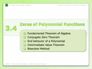
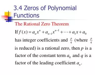
Graphing Polynomial Functions and Approximating Zeros • Look back in Chapter 4 to help with understanding finding zeros and the definition of even and odd functions • Location Principle: • If y = f(x) is a polynomial function and you have a and b such that f(a) < 0 and f(b) > 0 then there will be some number in between a and b that is a zero of the function • A relative maximum is the highest point between two zeros and a relative minimum is the lowest point between two zeros a zero b
Let’s use the table function on the graphing calculators combined with what we know about possible zeros. Graph the function f(x) = -2x3 – 5x2 + 3x + 2 and approximate the real zeros. There are zeros at approximately -2.9, -0.4, and -0.8.
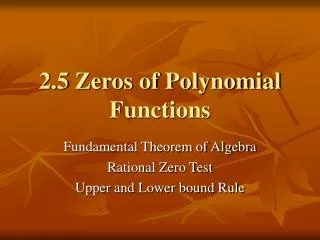
Upper Bound Theorem • If p(x) is divided by x – c and there are no sign changes in the quotient or remainder, then c is upper bound
. Lower Bound Theorem • If p(x) is divided by x + c and there are alternating sign changes in the quotient and the remainder, then -c is the lower bound.
Let’s put them to use… • Find an integral upper and lower bound of the zeros of