Download
1 / 35
350 likes | 502 Views
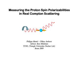
Measuring the Proton Spin Polarizabilities in Real Compton Scattering. Philippe Martel – UMass Amherst Advisor: Rory Miskimen TUNL (Triangle Universities Nuclear Lab) Bosen 2009. Table of Contents. Concerning spin-polarizabilities What are they? Where do they come from?

E N D
Measuring the Proton Spin Polarizabilities in Real Compton Scattering Philippe Martel – UMass Amherst Advisor: Rory Miskimen TUNL (Triangle Universities Nuclear Lab) Bosen 2009
Table of Contents • Concerning spin-polarizabilities • What are they? Where do they come from? • What is currently known? • Concerning the sensitivities to them • Observe changes in asymmetries after perturbing one • Smearing of effects from multiple perturbations • Concerning the fitting method • Constructing asymmetries and partials • Minimization checks • Results P. Martel - Bosen 2009
Nuclear Compton Scattering Compton scattering refers to scattering a photon off of a bound electron (atomic) or off of a nucleon (nuclear). Below about 20 MeV, this process is described by the Hamiltonian:* Above 20 MeV, the photon begins to probe the nucleon structure. To second order, an effective Hamiltonian can be written: Here, aE1 represents the electric, and bM1 the magnetic, dipole (scalar) polarizabilities.* *B. Holstein, GDH Convenor’s Report: Spin polarizabilities (2000) P. Martel - Bosen 2009
Spin Polarizabilities These scalar polarizabilities have been measured for the proton through real Compton scattering experiments.* Advancing to third order, four new terms arise in the eff. Hamiltonian:* These g terms are the spin (vector) polarizabilities. The subscript notation denotes their relation to a multipole expansion. *R.P. Hildebrandt, Elastic Compton Scattering from the Nucleon and Deuteron (2005) - Dissertation thesis P. Martel - Bosen 2009
S.P. Measurements The GDH experiments at Mainz and ELSA used the Gell-Mann, Goldberger, and Thirring sum rule to evaluate the forward S.P.: The Backward S.P. was determined from dispersive analysis of backward angle Compton scattering: *B. Pasquini et al., Proton Spin Polarizabilities from Polarized Compton Scattering (2007) P. Martel - Bosen 2009
S.P. Theoretical Values The pion-pole contribution has been subtracted from the experimental value for gp Calculations labeled O(pn) are ChPT LC3 and LC4 are O(p3) and O(p4) Lorentz invariant ChPT calculations SSE is small scale expansion Other calculations are dispersion theory Lattice QCD calculation by Detmold is in progress P. Martel - Bosen 2009
Dispersion Analysis Program The theoretical cross sections used here are produced in a fixed-t dispersion analysis code, provided to us by Barbara Pasquini. For further information, see B. Pasquini, D. Drechsel, M. Vanderhaeghen, Phys. Rev. C 76 015203 (2007). • The program was run for three different experimental runs: • Transversely polarized target with a circularly polarized beam • Longitudinally polarized target with a circularly polarized beam • Unpolarized target with a linearly polarized beam • The former two return cross sections for unpolarized, left helicity, and right helicity beams. The latter returns the beam asymmetry. P. Martel - Bosen 2009
Asymmetries After producing tables of cross sections with various values for the polarizabilities (their HDPV values, and those + 1 unit we construct the asymmetries: Using the counts, the statistical errors can be propagated through: P. Martel - Bosen 2009
S2x – g0 and gp Constrained P. Martel - Bosen 2009
S2z – g0 and gp Constrained P. Martel - Bosen 2009
S3 – g0 and gp Constrained P. Martel - Bosen 2009
S2x – All Four Multipole S.P.s P. Martel - Bosen 2009
S2z – All Four Multipole S.P.s P. Martel - Bosen 2009
S3 – All Four Multipole S.P.s P. Martel - Bosen 2009
Fitting Program • Cross sections → Counts → Asymmetries • Solid Angle of Detector • Real/Effective Polarization • Energy Bin Width • Partials with Respect to Polarizabilities • Pseudodata • 300 hours S2x, 300 hours S2z, 100 hours S3 • Fitting • c2 Construction • Minimization P. Martel - Bosen 2009
Solid Angle The solid angle for the chosen polar angle bin is given by: In order to tag the event (as likely described before), the reaction requires a proton recoil energy of at least 40 MeV, limiting our minimum forward angle of acceptance to: This, however, neglects the different events that different parts of the detector observe for a given run configuration, which will be corrected for in the next section. P. Martel - Bosen 2009
Real/Effective Polarization The cross sections produced in the code assume 100% beam and target polarization (if applicable). The cross sections with a real polarization: For S2x and S3 Transversely Longitudinally Unpolarized Where red is target polarization, and gray is beam polarization direction P. Martel - Bosen 2009
Real/Effective Polarization The effective polarizations can then be written as: With the expected experimental polarizations, the resulting effective polarizations are: P. Martel - Bosen 2009
Minimization Partials The energy bin averaged counts can be written in a linear expansion: Where kmax, kmin, and k0 are the energy bin max, min, and centroid respectively, Dgi is the S.P. perturbation, and F is the flux factor: The Ci term represents the partials of the counts with respect to the S.P.s P. Martel - Bosen 2009
c2 Construction The fitting program uses a minimization routine on c2, defined as: The algorithm is actually the summation of various c2components, including the selected constraints for the particular run. Is it reasonable, however, to assume that the theoretical component can be approximated by a linear expansion? Run a c2 check. P. Martel - Bosen 2009
c2 Check – 240 MeV P. Martel - Bosen 2009
c2 Check – 280 MeV P. Martel - Bosen 2009
S.P. Fitting – 240 MeV (g0, gp con.) P. Martel - Bosen 2009
Con. Values – 240 MeV (g0, gp con.) P. Martel - Bosen 2009
S.P. Fitting – 240 MeV (no g con.) P. Martel - Bosen 2009
Con. Values – 240 MeV (no g con.) P. Martel - Bosen 2009
S.P. Fitting – 280 MeV (g0, gp con.) P. Martel - Bosen 2009
Con. Values – 280 MeV (g0, gp con.) P. Martel - Bosen 2009
S.P. Fitting – 280 MeV (no g con.) P. Martel - Bosen 2009
Con. Values – 280 MeV (no g con.) P. Martel - Bosen 2009
Results The tabulated results for running with both the g0 and gp constraints: The tabulated results for running with no g constraints: P. Martel - Bosen 2009
Conclusions • By simply plotting the changes in the asymmetries, the sensitivities to the polarizabilities is seen to be appreciable. • Checks of the fitting method being used demonstrates reasonable behavior (near linearity and containment) • Fitting results are very promising: • Running the full program with S2x, S2z, and S3 appears to be sufficient to extract the S.P.s without invoking the g0 or gp constraints. • This would provide the first set of experimental values for these important quantities! P. Martel - Bosen 2009