Download
1 / 25
370 likes | 514 Views
Delve into the world of cosmological simulations to enhance our knowledge of the universe, confront complex models computationally, and visualize unobservable phenomena. Discover the collisionless dynamics and fluid simulation techniques used, along with the challenges, theoretical basis, and equations of motion involved. Explore N-body methods, theoretical assumptions, and various mesh and tree methodologies applied in these simulations.

E N D
Motivation • Improve our understanding of the universe • Reason about models that are intractable from an analytic point of view • Verify/compare different models/theories by simulating them computationally and comparing to observational results. • Ex: the Lambda-Cold Dark Matter model developed into the leading theoretical paradigm of structure formation in large part because of simulation results • Create visualizations of distant/unobservable phenomena.
Challenges • The N-body problem is PSPACE-hard • Modelling the universe takes an enormous amount of computation • Until recently, could only perform very small simulations • Advances in hardware and methods allow us to simulate much larger systems much more accurately
Methodology • Most simulations need to describe 2 primary components: • Collisionless dynamics (dark matter and stars in galaxies) • Fluid simulation of an ideal gas (baryonic matter, primarily hydrogen and helium) • Require a solve method for each of these two components to accurately simulate the universe • Additional physics may be optionally added (radiative cooling, star formation methods, cosmic rays, supermassive black hole growth, stellar winds, etc.)
Collisionless Dynamics • Best solved by N-body methods, where space is sampled with a finite number of tracer particles • Difficulty: the number of interactions increases with N2, which can be very expensive • Main forms of approximating the simulation: • Particle mesh methods • Tree methods • Hybrid
Theoretical Basis • Assumption is that dark matter does not interact appreciably except through gravity. • In order for the collisionless assumption to hold, simulation time should be much shorter than relaxation time • For galaxy clusters, this time period is on the order of 1012 years, or 100 times the age of the universe • Simplifying assumption: dark matter particles (which constitute the vast majority of this category) only interact via gravity
Equations of Motion • Collisionless Boltzmann Equation: • is the gravitational field potential • Poisson Equation: • is the single particle distribution function • Solution for the Equations of Motion: • is a gravitational softening constant; prevents large angle scattering and bound pairs, and assures that the two-body relaxation time is large; allows low order integration
Particle Mesh Methods • System of particles converted into a grid of density values • Forces are applied to a body based on which cell it is in, and where in the cell it is • Particles do not interact directly, but rather through a mean field • Typically solved via Fast Fourier Transform • Time is linear in particles and O(n log n) in cells • Fastest method available, but force is suppressed below one to two mesh cells; leads to bad spatial accuracy
Tree Methods • Recursively divide the N bodies into groups • Each node represents a region (root is the whole simulation) • For an internal node whose center of mass is sufficiently far from a body being simulated, the entire node is treated as a single body with mass equal to the total mass of the bodies under the node • O(n log n) time in number of particles • Much better accuracy, but also much slower
Hybrid Methods • Tree – PM: • Restrict the tree algorithm to short-range scales • Uses particle mesh method to compute long-range gravitational force • Most commonly used method today; very well suited for cosmological simulation (available in both GADGET and AREPO)
Fluid Simulation (Basic Methods) • Eulerian (mesh): discretize space and represent fluid variables on a mesh • Very good for capturing hydrodynamical shocks • Suboptimal for the large dynamic range inherent in cosmology • Can’t track history of individual fluid elements • Adaptive Mesh Refinement is used in modern implementations • Lagrangian (SPH): discretize mass using a set of fluid particles (used in the GADGET code) • Well suited to follow gravitational growth of structure • Automatically increase resolution in critical regions • Does not handle shocks well: relies on injection of artificial viscosity • Can’t represent the discontinuous nature of shocks (due to smoothing) • Both widely used
Fluid Simulation (Moving Mesh) • Uses unstructured mesh defined by Voronoi tessellation of a set of points • The points are allowed to move with the fluid to give accuracy where it is needed • Can be thought of as a sort of hybrid between AMR and SPH • Mitigates the noise and diffusiveness of SPH • Handles self-gravity better than AMR
Fluid Simulation (Moving Mesh) • The mesh is defined by a set of points • If the points are fixed, then the method is the standard Eulerian method • If the points are allowed to move freely with the fluid being simulated, then it becomes a Lagrangian method • There is usually a correction factor to prevent the mesh from over-distorting: • Threshold of the density of the cells • Threshold of the distance between the geometric distance from the center of the cell to the point • Threshold the angle between the cell walls
Integration • Adaptive timesteps given by • is an accuracy parameter, is the gravitational softening, and is the acceleration of the particle
Current State of the Art Methods • SPH-based method: GADGET (2001) / GADGET-II (2005) • Moving mesh method: AREPO (2009) • These two currently dominate most large-scale simulation tasks in cosmology.
GADGET / GADGET-II • One of the most widely used simulation programs • Uses smoothed particle hydrodynamics for fluid simulation • Introduced use of entropy as an independent variable in fluid simulation • Improved on time-step implementation
AREPO • Relatively new implementation • Uses moving mesh methods for fluid simulation • Can refine/de-refine the mesh cells based on density • Has begun to gain widespread use • Is slightly slower than GADGET-II, but has been shown to be more accurate in many applications • Angular momentum is modelled more accurately • Gas mixture handled more efficiently, which models the cooling of hot halos more accurately • Does not show clumps due to cooling instability
Notable Simulations • Millenium (2005) • Bolshoi (2010) • Illustris (2014)
Millenium • Completed in 2005, first truly gigantic cosmological simulation • Simulates from the epoch when the cosmic background radiation was emitted • Traced 10 billion particles across a cubic region of space 2 billion light years in length • Ran using the GADGET code on a supercomputer for over a month, producing 25 terabytes of data • The data has been used in over 650 papers • One of the highest impact astronomy simulations • Initial results were able to reconcile observations by the Sloan Digital Sky Survey (SDSS) with model of the universe • SDSS observed very bright quasars at large distances, which implied that they were formed much earlier than originally theorized; this challenged then-current understanding of cosmology • Simulation was able to reproduce the early formation of such quasars and showed that these objects are not at odds with our models of the universe
Bolshoi Simulation • Completed in 2010 • At the time, it was the most accurate simulation of the evolution of the large scale structure of the universe • Traced 8.6 billion particles of dark matter across a cubic region of space 1 billion light years in length • Ran using a adaptive mesh refinement method called Adaptive Refinement Tree • Used density as decision factor for subdividing • Neighboring cells are kept to within one subdivision level of each other to prevent discontinuity • Very close agreement with SDSS observations
Illustris • Completed in 2014 • Uses the AREPO moving mesh code • Follows 18 billion particles on a ~350 million light year cube • Results are still being released • Initial results show very good agreement with observable metrics in: • Ratio of dark matter to baryonic matter • Star formation rate • Distributions of various types/sizes of galaxies • Gas distribution
References • http://www.mpa-garching.mpg.de/gadget/ • http://www.mpa-garching.mpg.de/~volker/arepo/ • http://www.mpa-garching.mpg.de/millennium/ • http://hipacc.ucsc.edu/Bolshoi/ • http://www.illustris-project.org/ • http://www.cfa.harvard.edu/itc/research/movingmeshcosmology/ • http://obswww.unige.ch/lastro/conferences/sf2013/pdf/lecture1.pdf • http://www.scholarpedia.org/article/N-body_simulations • http://www.usm.uni-muenchen.de/people/puls/lessons/numpraktnew/nbody/nbody_manual.pdf