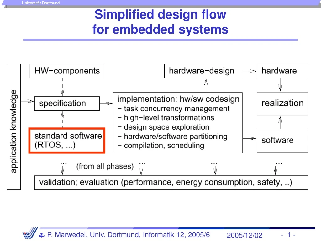
Simplified design flow for embedded systems

1. Simplified design flowfor embedded systems 2005/12/02

2. Reuse of standard software components • Knowledge from previous designs to bemade available in the form of intellectualproperty (IP, for SW & HW). • Operating systems • Middleware • Real-time data bases • Standard software (MPEG-x, GSM-kernel, …) • Includes standard approaches for scheduling • (requires knowledge about execution times).

3. Worst/best case execution times (1) • Def.: The worst case execution time (WCET) is an upper bound on the execution times of tasks. • The term is not ideal, since a program requiring the WCET for its execution does not have to exist (WCET is a bound). Def.: The best case execution time (BCET) is a lower bound on the execution times of tasks. The term is not ideal, since a program running at the BCET for its execution does not have to exist (BCET is a bound).

4. Worst/best case execution times (2) Actually best possible ex. time Actually possible worst case Definition used in this course Observed execution time WCET’ (tighter bound) BCET' BCET WCET Feasibleexecutiontimes t Other authors WCET BCET Observed WCET Estimated WCET EstimatedBCET Feasible execution times

5. Worst case execution times (2) • Complexity: • in the general case: undecidable if a bound exists. • for restricted programs: simple for „old“ architectures,very complex for new architectures with pipelines, caches, interrupts, virtual memory, etc. • Approaches: • for hardware: requires detailed timing behavior • for software: requires availability of machine programs;complex analysis (see, e.g., www.absint.de)

6. π x • Accurate cost and performance values:Can be done with normal tools(such as compilers).As precise as the input data is. Average execution times • Estimated cost and performance values:Difficult to generate sufficiently precise estimates;Balance between run-time and precision

7. Real-time scheduling (1) • Assume that we are given a task graph G=(V,E). • Def.: A schedules of G is a mapping V  Tof a set of tasks V to start times from domain T. V3 V4 G=(V,E) V1 V2 s T t

8. Real-time scheduling (2) • Typically, schedules have to respect a number of constraints, incl. resource constraints, dependency constraints, deadlines. • Scheduling = finding such a mapping. • Scheduling to be performed several times during ES design (early rough scheduling as well as late precise scheduling).

9. Classification of scheduling algorithms

10. Hard and soft deadlines • Def.: A time-constraint (deadline) is called hard if not meeting that constraint could result in a catastrophe [Kopetz, 1997]. • All other time constraints are called soft. • We will focus on hard deadlines.

11. Periodic and aperiodic tasks • Def.: Tasks which must be executed once every p units of time are called periodic tasks. p is called their period. Each execution of a periodic task is called a job. • All other tasks are called aperiodic. • Def.: Tasks requesting the processor at unpredictable times are called sporadic, if there is a minimum separation between the times at which they request the processor.

12. Preemptive and non-preemptive scheduling • Non-preemptive schedulers:Tasks are executed until they are done.Response time for external events may be quite long. • Preemptive schedulers: To be used if • some tasks have long execution times or • if the response time for external events to be short.

13. Dynamic/online scheduling • Dynamic/online scheduling:Processor allocation decisions (scheduling) at run-time; based on the information about the tasks arrived so far.

14. Static/offline scheduling • Static/offline scheduling:Scheduling taking a priori knowledge about arrival times, execution times, and deadlines into account.Dispatcher allocates processor when interrupted by timer. Timer controlled by a table generated at design time.

15. Time-triggered systems (1) • In an entirely time-triggered system, the temporal control structure of all tasks is established a priori by off-line support-tools. This temporal control structure is encoded in a Task-Descriptor List (TDL) that contains the cyclic schedule for all activities of the node. This schedule considers the required precedence and mutual exclusion relationships among the tasks such that an explicit coordination of the tasks by the operating system at run time is not necessary. .. • The dispatcher is activated by the synchronized clock tick. It looks at the TDL, and then performs the action that has been planned for this instant [Kopetz].

16. Time-triggered systems (2) • … pre-run-time scheduling is often the only practical means of providing predictability in a complex system. [Xu, Parnas]. • It can be easily checked if timing constraints are met. The disadvantage is that the response to sporadic events may be poor.

17. Centralized and distributed scheduling • Centralized and distributed scheduling:Multiprocessor scheduling either locally on 1 or on several processors. • Mono- and multi-processor scheduling: • Simple scheduling algorithms handle single processors, • more complex algorithms handle multiple processors. • algorithms for homogeneous multi-processor systems • algorithms for heterogeneous multi-processor systems (includes HW accelerators as special case).

18. Schedulability • Set of tasks is schedulable under a set of constraints, if a schedule exists for that set of tasks & constraints. • Exact tests are NP-hard in many situations. • Sufficient tests: sufficient conditions for schedule checked. (Hopefully) small probability of indicating that no schedule exists even though one exists. • Necessary tests: checking necessary conditions. Used to show no schedule exists. There may be cases in which no schedule exists & we cannot prove it. necessary schedulable sufficient

19. T1 T2 Max. lateness t Cost functions • Cost function: Different algorithms aim at minimizing different functions. • Def.: Maximum lateness = maxall tasks(completion time – deadline) Is <0 if all tasks complete before deadline.

20. Simple tasks • Tasks without any interprocess communication are called simple tasks (S-tasks). • S-tasks can be in one out of two states: ready or running. ready running

21. Simple tasks • The API of a TT-OS supporting S-tasks is .. simple [Kopetz]: • It consists of 3 data structures & 2 OS calls. ... The calls are TERMINATE TASK & ERROR. • The TERMINATE TASK system call is executed whenever the task has reached its termination point. • In case of an error that cannot be handled within the application task, the task terminates its operation with the ERROR system call. ready running

22. ℓi Aperiodic scheduling- Scheduling with no precedence constraints - • Let {Ti} be a set of tasks. Let: • ci be the execution time of Ti , • di be the deadline interval, that is, the time between Ti becoming available and the time until which Ti has to finish execution. • ℓi be the laxity or slack,defined asℓi = di - ci • fi be the finishing time.

23. Uniprocessor with equal arrival times • Preemption is useless. • Earliest Due Date (EDD): Execute task with earliest due date (deadline) first. fi fi fi EDD requires all tasks to be sorted by their (absolute) deadlines. Hence, its complexity is O(n log(n)).

24. Morein-depth: Optimality of EDD • EDD is optimal, since it follows Jackson's rule:Given a set of n independent tasks, any algorithm that executes the tasks in order of non-decreasing (absolute) deadlines is optimal with respect to minimizing the maximum lateness. • Proof (See Buttazzo, 2002): • Let  be a schedule produced by any algorithm A • If A  EDD   Ta, Tb, da≤ db, Tb immediately precedes Tb in . • Let ' be the schedule obtained by exchanging Ta andTb.

25. Exchanging Ta and Tb cannot increase lateness • Max. lateness for Ta and Tb in  is Lmax(a,b)=fa-da Max. lateness for Ta and Tb in ' is L'max(a,b)=max(L'a,L'b) • Two possible cases • L'a ≥L'b: L'max(a,b) = f'a – da < fa – da =Lmax(a,b)since Ta starts earlier in schedule '. • L'a ≤L'b:  L'max(a,b) = f'b – db = fa – db ≤ fa – da = Lmax(a,b) since fa=f'b and da≤ db •  L'max(a,b) ≤ Lmax(a,b)  Tb Ta ' Ta Tb fa=f'b

26. end EDD is optimal • Any schedule  with lateness L can be transformed into an EDD schedule n with lateness Ln≤ L, which is the minimum lateness. • EDD is optimal (q.e.d.)

27. Earliest Deadline First (EDF)- Horn’s Theorem - • Different arrival times: Preemption potentially reduces lateness. • Theorem [Horn74]: Given a set of n independent tasks with arbitrary arrival times, any algorithm that at any instant executes the task with the earliest absolute deadline among all the ready tasks is optimal with respect to minimizing the maximum lateness.

28. Earliest Deadline First (EDF)- Algorithm - • Earliest deadline first (EDF) algorithm: Each time a new ready task arrives: • It is inserted into a queue of ready tasks, sorted by their absolute deadlines. Task at head of queue is executed. • If a newly arrived task is inserted at the head of the queue, the currently executing task is preempted. • Straightforward approach with sorted lists (full comparison with existing tasks for each arriving task) requires run-time O(n2); (less with binary search or bucket arrays). Sorted queue Executing task

29. Earliest Deadline First (EDF)- Example - Later deadline  no preemption Earlier deadline preemption

30. Least laxity (LL), Least Slack Time First (LST) • Priorities = decreasing function of the laxity (the less laxity, the higher the priority); dynamically changing priority; preemptive.

31. Properties • Not sufficient to call scheduler & re-compute laxity just at task arrival times. • Overhead for calls of the scheduler. • Many context switches. • Detects missed deadlines early. • LL is also an optimal scheduling for mono-processor systems. • Dynamic priorities  cannot be used with a fixed prio OS. • LL scheduling requires the knowledge of the execution time.

32. Scheduling without preemption Lemma: If preemption is not allowed, optimal schedules may have to leave the processor idle at certain times. Proof: Suppose: optimal schedulers never leave processor idle.

33. Scheduling without preemption (2) • T1: periodic, c1 = 2, p1 = 4, d1 = 4 • T2: occasionally available at times 4*n+1, c2= 1, d2= 1 • T1 has to start at t=0 •  deadline missed, but schedule is possible (start T2 first) •  scheduler is not optimal  contradiction! q.e.d.

34. Scheduling without preemption • Preemption not allowed:  optimal schedules may leave processor idle to finish tasks with early deadlines arriving late. • Knowledge about the future is needed for optimal scheduling algorithmsNo online algorithm can decide whether or not to keep idle. • EDF is optimal among all scheduling algorithms not keeping the processor idle at certain times. • If arrival times are known a priori, the scheduling problem becomes NP-hard in general. B&B typically used.

35. Scheduling with precedence constraints • Task graph and possible schedule: Schedule can be stored in table.

36. Simultaneous Arrival Times:The Latest Deadline First (LDF) Algorithm • LDF [Lawler, 1973]: reads the task graph and among the tasks with no successors inserts the one with the latest deadline into a queue. It then repeats this process, putting tasks whose successor have all been selected into the queue. • At run-time, the tasks are executed in the generated total order. • LDF is non-preemptive and is optimal for mono-processors. If no local deadlines exist, LDF performs just a topological sort.

37. Asynchronous Arrival Times:Modified EDF Algorithm • This case can be handled with a modified EDF algorithm.The key idea is to transform the problem from a given set of dependent tasks into a set of independent tasks with different timing parameters [Chetto90]. • This algorithm is optimal for mono-processor systems. • If preemption is not allowed, the heuristic algorithm developed by Stankovic and Ramamritham can be used.

38. Summary • Worst case execution times (WCET) • Definition of scheduling terms • Hard vs. soft deadlines • Static vs. dynamic TT-OS • Schedulability • Scheduling approaches • Aperiodic tasks • No precedences • Simultaneous (EDD) & Asynchronous Arrival Times (EDF, LL) • Precedences • Simultaneous ( LDF) & Asynchronous Arrival Times ( mEDF)