Download
1 / 60
670 likes | 1.21k Views
Asset Pricing Models Learning Objectives. 1. Assumptions of the capital asset pricing model 2. Markowitz efficient frontier 3. Risk-free asset and its risk-return characteristics 4. Combining the risk-free asset with portfolio of risky assets on the efficient frontier.

E N D
Asset Pricing ModelsLearning Objectives 1. Assumptions of the capital asset pricing model 2. Markowitz efficient frontier 3. Risk-free asset and its risk-return characteristics 4. Combining the risk-free asset with portfolio of risky assets on the efficient frontier
Asset Pricing ModelsLearning Objectives 5. The market portfolio 6. What is the capital market line (CML)? 7. How to measure diversification for an individual portfolio? 8. Systematic Vs. unsystematic risk 9. Security market line (SML) and how does it differ from the CML? 10. Determining undervalued and overvalued security
Capital Market Theory: An Overview • Capital market theory extends portfolio theory and develops a model for pricing all risky assets • Capital asset pricing model (CAPM) will allow you to determine the required rate of return for any risky asset
Assumptions of Capital Market Theory 1. All investors are Markowitz efficient 2. Borrowing or lending at the risk-free rate 3. Homogeneous expectations 4. One-period time horizon 5. Investments are infinitely divisible 6. No taxes or transaction costs 7. Inflation is fully anticipated 8. Capital markets are in equilibrium.
Assumptions of Capital Market Theory 1. All investors are Markowitz efficient investors who want to target points on the efficient frontier. • The exact location on the efficient frontier and, therefore, the specific portfolio selected, will depend on the individual investor’s risk-return utility function.
Assumptions of Capital Market Theory 2. Investors can borrow or lend any amount of money at the risk-free rate of return (RFR). • Clearly it is always possible to lend money at the nominal risk-free rate by buying risk-free securities such as government T-bills. It is not always possible to borrow at this risk-free rate, but we will see that assuming a higher borrowing rate does not change the general results.
Assumptions of Capital Market Theory 3. All investors have homogeneous expectations; that is, they estimate identical probability distributions for future rates of return. • Again, this assumption can be relaxed. As long as the differences in expectations are not vast, their effects are minor.
Assumptions of Capital Market Theory 4. All investors have the same one-period time horizon such as one-month, six months, or one year. • The model will be developed for a single hypothetical period, and its results could be affected by a different assumption. A difference in the time horizon would require investors to derive risk measures and risk-free assets that are consistent with their time horizons.
Assumptions of Capital Market Theory 5. All investments are infinitely divisible, which means that it is possible to buy or sell fractional shares of any asset or portfolio. • This assumption allows us to discuss investment alternatives as continuous curves. Changing it would have little impact on the theory.
Assumptions of Capital Market Theory 6. There are no taxes or transaction costs involved in buying or selling assets. • This is a reasonable assumption in many instances. Neither pension funds nor religious groups have to pay taxes, and the transaction costs for most financial institutions are less than 1 percent on most financial instruments. Again, relaxing this assumption modifies the results, but does not change the basic thrust.
Assumptions of Capital Market Theory 7. There is no inflation or any change in interest rates, or inflation is fully anticipated. • This is a reasonable initial assumption, and it can be modified.
Assumptions of Capital Market Theory 8. Capital markets are in equilibrium. • This means that we begin with all investments properly priced in line with their risk levels.
Assumptions of Capital Market Theory • Some of these assumptions are unrealistic • Relaxing many of these assumptions would have only minor influence on the model and would not change its main implications or conclusions. • A theory should be judged on how well it explains and helps predict behavior, not on its assumptions.
The Efficient Frontier • The efficient frontier represents that set of portfolios with the maximum rate of return for every given level of risk, or the minimum risk for every level of return • Frontier will be portfolios of investments rather than individual securities • Exceptions being the asset with the highest return and the asset with the lowest risk
Efficient Frontier for Alternative Portfolios Exhibit 7.15 Efficient Frontier B E(R) A C Standard Deviation of Return
Risk-Free Asset • An asset with zero standard deviation • Zero correlation with all other risky assets • Provides the risk-free rate of return (RFR) • Will lie on the vertical axis of a portfolio graph
Risk-Free Asset Covariance between two sets of returns is Because the returns for the risk free asset are certain, Thus Ri = E(Ri), and Ri - E(Ri) = 0 Consequently, the covariance of the risk-free asset with any risky asset or portfolio will always equal zero. Similarly the correlation between any risky asset and the risk-free asset would be zero.
Combining a Risk-Free Asset with a Risky Portfolio Expected return the weighted average of the two returns This is a linear relationship
Combining a Risk-Free Asset with a Risky Portfolio Standard deviation The expected variance for a two-asset portfolio is Substituting the risk-free asset for Security 1, and the risky asset for Security 2, this formula would become Since we know that the variance of the risk-free asset is zero and the correlation between the risk-free asset and any risky asset i is zero we can adjust the formula
Combining a Risk-Free Asset with a Risky Portfolio Given the variance formula the standard deviation is Therefore, the standard deviation of a portfolio that combines the risk-free asset with risky assets is the linear proportion of the standard deviation of the risky asset portfolio.
Combining a Risk-Free Asset with a Risky Portfolio Since both the expected return and the standard deviation of return for such a portfolio are linear combinations, a graph of possible portfolio returns and risks looks like a straight line between the two assets.
Portfolio Possibilities Combining the Risk-Free Asset and Risky Portfolios on the Efficient Frontier Exhibit 8.1 D M C B A RFR
Risk-Return Possibilities with Leverage To attain a higher expected return than is available at point M (in exchange for accepting higher risk) • Either invest along the efficient frontier beyond point M, such as point D • Or, add leverage to the portfolio by borrowing money at the risk-free rate and investing in the risky portfolio at point M
Portfolio Possibilities Combining the Risk-Free Asset and Risky Portfolios on the Efficient Frontier CML Borrowing Lending Exhibit 8.2 M RFR
The Market Portfolio • Because portfolio M lies at the point of tangency, it has the highest portfolio possibility line • Everybody will want to invest in Portfolio M and borrow or lend to be somewhere on the CML • Therefore this portfolio must include ALL RISKY ASSETS
The Market Portfolio • Because the market is in equilibrium, all assets are included in this portfolio in proportion to their market value • Because it contains all risky assets, it is a completely diversified portfolio, which means that all the unique risk of individual assets (unsystematic risk) is diversified away
Systematic Risk • Only systematic risk remains in the market portfolio • Systematic risk is the variability in all risky assets caused by macroeconomic variables • Systematic risk can be measured by the standard deviation of returns of the market portfolio and can change over time
How to Measure Diversification • All portfolios on the CML are perfectly positively correlated with each other and with the completely diversified market Portfolio M • A completely diversified portfolio would have a correlation with the market portfolio of +1.00
Diversification and the Elimination of Unsystematic Risk • The purpose of diversification is to reduce the standard deviation of the total portfolio • This assumes that imperfect correlations exist among securities • As you add securities, you expect the average covariance for the portfolio to decline • How many securities must you add to obtain a completely diversified portfolio?
Number of Stocks in a Portfolio and the Standard Deviation of Portfolio Return Standard Deviation of Return Exhibit 8.3 Unsystematic (diversifiable) Risk Total Risk Standard Deviation of the Market Portfolio (systematic risk) Systematic Risk Number of Stocks in the Portfolio
A Risk Measure for the CML • Covariance with the M portfolio is the systematic risk of an asset • The Markowitz portfolio model considers the average covariance with all other assets in the portfolio • The only relevant portfolio is the M portfolio
A Risk Measure for the CML Together, this means the only important consideration is the asset’s covariance with the market portfolio
A Risk Measure for the CML Because all individual risky assets are part of the M portfolio, an asset’s rate of return in relation to the return for the M portfolio may be described using the following linear model: where: Rit = return for asset i during period t ai = constant term for asset i bi = slope coefficient for asset i RMt = return for the M portfolio during period t = random error term
The Capital Asset Pricing Model: Expected Return and Risk • The existence of a risk-free asset resulted in deriving a capital market line (CML) that became the relevant frontier • An asset’s covariance with the market portfolio is the relevant risk measure • This can be used to determine an appropriate expected rate of return on a risky asset - the capital asset pricing model (CAPM)
The Capital Asset Pricing Model: Expected Return and Risk • CAPM indicates what should be the expected or required rates of return on risky assets • This helps to value an asset by providing an appropriate discount rate to use in dividend valuation models • You can compare an estimated rate of return to the required rate of return implied by CAPM - over/under valued ?
The Security Market Line (SML) • The relevant risk measure for an individual risky asset is its covariance with the market portfolio (Covi,m) • This is shown as the risk measure • The return for the market portfolio should be consistent with its own risk, which is the covariance of the market with itself - or its variance:
Exhibit 8.5 Graph of Security Market Line (SML) SML RFR
The Security Market Line (SML) The equation for the risk-return line is We then define as beta
Exhibit 8.6 Graph of SML with Normalized Systematic Risk SML Negative Beta RFR
Determining the Expected Rate of Return for a Risky Asset • The expected rate of return of a risk asset is determined by the RFR plus a risk premium for the individual asset • The risk premium is determined by the systematic risk of the asset (beta) and the prevailing market risk premium (RM-RFR)
Determining the Expected Rate of Return for a Risky Asset Assume: RFR = 6% (0.06) RM = 12% (0.12) Implied market risk premium = 6% (0.06) E(RA) = 0.06 + 0.70 (0.12-0.06) = 0.102 = 10.2% E(RB) = 0.06 + 1.00 (0.12-0.06) = 0.120 = 12.0% E(RC) = 0.06 + 1.15 (0.12-0.06) = 0.129 = 12.9% E(RD) = 0.06 + 1.40 (0.12-0.06) = 0.144 = 14.4% E(RE) = 0.06 + -0.30 (0.12-0.06) = 0.042 = 4.2%
Determining the Expected Rate of Return for a Risky Asset • In equilibrium, all assets and all portfolios of assets should plot on the SML • Any security with an estimated return that plots above the SML is underpriced • Any security with an estimated return that plots below the SML is overpriced • A superior investor must derive value estimates for assets that are consistently superior to the consensus market evaluation to earn better risk-adjusted rates of return than the average investor
Identifying Undervalued and Overvalued Assets • Compare the required rate of return to the expected rate of return for a specific risky asset using the SML over a specific investment horizon to determine if it is an appropriate investment • Independent estimates of return for the securities provide price and dividend outlooks
Price, Dividend, and Rate of Return Estimates Exhibit 8.7
Comparison of Required Rate of Return to Estimated Rate of Return Exhibit 8.8
The Effect of the Market Proxy • The market portfolio of all risky assets must be represented in computing an asset’s characteristic line • Standard & Poor’s 500 Composite Index is most often used • Large proportion of the total market value of U.S. stocks • Value weighted series
Weaknesses of Using S&P 500as the Market Proxy • Includes only U.S. stocks • The theoretical market portfolio should include U.S. and non-U.S. stocks and bonds, real estate, coins, stamps, art, antiques, and any other marketable risky asset from around the world
Differential Borrowing and Lending Rates Heterogeneous Expectations and Planning Periods Zero Beta Model does not require a risk-free asset Transaction Costs with transactions costs, the SML will be a band of securities, rather than a straight line Relaxing the Assumptions
Heterogeneous Expectations and Planning Periods will have an impact on the CML and SML Taxes could cause major differences in the CML and SML among investors Relaxing the Assumptions