
提问:数值分析是做什么用的?
提问:数值分析是做什么用的?. 数值 分析. 输入复杂问题或运算. 计算机. 近似解. . 第一章 误差 /* Error */. §1 误差的背景介绍 /* Introduction */. 1. 来源与分类 /* Source & Classification */. 从实际问题中抽象出数学模型 —— 模型误差 /* Modeling Error */. 通过测量得到模型中参数的值 —— 观测误差 /* Measurement Error */.

提问:数值分析是做什么用的?
E N D
Presentation Transcript
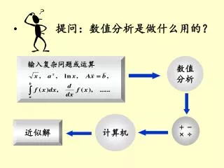
提问:数值分析是做什么用的? 数值 分析 输入复杂问题或运算 计算机 近似解
第一章 误差 /* Error */ §1 误差的背景介绍 /* Introduction */ 1. 来源与分类 /* Source & Classification */ • 从实际问题中抽象出数学模型 —— 模型误差 /* Modeling Error */ • 通过测量得到模型中参数的值 —— 观测误差 /* Measurement Error */ • 求近似解 —— 方法误差 (截断误差 /* Truncation Error */ ) • 机器字长有限 —— 舍入误差/* Roundoff Error */
§1 Introduction: Source & Classification The following problem can be solved either the easy way or the hard way. Two trains 200 miles apart are moving toward each other; each one is going at a speed of 50 miles per hour. A fly starting on the front of one of them flies back and forth between them at a rate of 75 miles per hour. It does this until the trains collide and crush the fly to death. What is the total distance the fly has flown? The fly actually hits each train an infinite number of times before it gets crushed, and one could solve the problem the hard way with pencil and paper by summing an infinite series of distances. The easy way is as follows: Since the trains are 200 miles apart and each train is going 50 miles an hour, it takes 2 hours for the trains to collide. Therefore the fly was flying for two hours. Since the fly was flying at a rate of 75 miles per hour, the fly must have flown 150 miles. That's all there is to it. When this problem was posed to John von Neumann, he immediately replied, "150 miles." "It is very strange," said the poser, "but nearly everyone tries to sum the infinite series." "What do you mean, strange?" asked Von Neumann. "That's how I did it!"
§1 Introduction: Source & Classification 例:近似计算 大家一起猜? 取 S4 R4/* Remainder */ 则 称为截断误差 /* Truncation Error */ 解法之一:将 作Taylor展开后再积分 |舍入误差/* Roundoff Error */ | = 0.747… … 1 / e 1 由留下部分 /* included terms */ 引起 由截去部分 /* excluded terms */ 引起
据说,美军 1910 年的一次部队的命令传递是这样的: 营长对值班军官: 明晚大约 8点钟左右,哈雷彗星将可能在这个地区看到,这种彗星每隔 76年才能看见一次。命令所有士兵着野战服在操场上集合,我将向他们解释这一罕见的现象。如果下雨的话,就在礼堂集合,我为他们放一部有关彗星的影片。 值班军官对连长: 根据营长的命令,明晚8点哈雷彗星将在操场上空出现。如果下雨的话,就让士兵穿着野战服列队前往礼堂,这一罕见的现象将在那里出现。 连长对排长: 根据营长的命令,明晚8点,非凡的哈雷彗星将身穿野战服在礼堂中出现。如果操场上下雨,营长将下达另一个命令,这种命令每隔76年才会出现一次。 排长对班长: 明晚8点,营长将带着哈雷彗星在礼堂中出现,这是每隔 76年才有的事。如果下雨的话,营长将命令彗星穿上野战服到操场上去。 班长对士兵: 在明晚8点下雨的时候,著名的76岁哈雷将军将在营长的陪同下身着野战服,开着他那“彗星”牌汽车,经过操场前往礼堂。
§1 Introduction: Spread & Accumulation 2. 传播与积累 /* Spread & Accumulation */ 例:蝴蝶效应—— 纽约的一只蝴蝶翅膀一拍,风和日丽的北京就刮起台风来了?! NY BJ 以上是一个病态问题/* ill-posed problem*/ 关于本身是病态的问题,我们还是留给数学家去头痛吧!
§1 Introduction: Spread & Accumulation 例:计算 公式一: 则初始误差 记为 注意此公式精确成立 What happened?! ? ?? ? ! ! !
§1 Introduction: Spread & Accumulation 考察第n步的误差 可见初始的小扰动 迅速积累,误差呈递增走势。 造成这种情况的是不稳定的算法 /* unstable algorithm */ 我们有责任改变。 公式二: 可取 方法:先估计一个IN,再反推要求的In ( n << N )。 注意此公式与公式一 在理论上等价。
§1 Introduction: Spread & Accumulation 取 We just got lucky?
§1 Introduction: Spread & Accumulation 考察反推一步的误差: 以此类推,对 n < N有: 误差逐步递减, 这样的算法称为稳定的算法 /* stable algorithm */ 在我们今后的讨论中,误差将不可回避, 算法的稳定性会是一个非常重要的话题。
其中x为精确值,x*为x的近似值。 的上限记为 ,称为绝对误差限/* accuracy */, Oh yeah? Then tell me the absolute error of 工程上常记为 ,例如: §2误差与有效数字 /* Error and Significant Digits */ 绝对误差 /* absolute error */ Hey isn’t it simple? 注:e* 理论上讲是唯一确定的,可能取正,也可能取负。 e* > 0 不唯一,当然 e* 越小越具有参考价值。 Oops! Of course mine is more accurate ! The accuracy relates to not only the absolute error, but also to the size of the exact value. I can tell that distance between two planets is 1 million light year ±1 light year. I can tell that this part’s diameter is 20cm1cm.
§2 Error and Significant Digits A mathematician, a physicist, and an engineer were traveling through Scotland when they saw a black sheep through the window of the train. "Aha," says the engineer, "I see that Scottish sheep are black." "Hmm," says the physicist, "You mean that some Scottish sheep are black." "No," says the mathematician, "All we know is that there is at least one sheep in Scotland, and that at least one side of that one sheep is black!" x 的相对误差上限/* relative accuracy */定义为 注:从 的定义可见, 实际上被偷换成了 ,而后才考察其上限。那么这样的偷换是否合法? 严格的说法是, 与 是否反映了同一数量级的误差? 关于此问题的详细讨论可见教材第3页。 相对误差 /* relative error */ Now I wouldn’t call it simple. Say … what is the relative error of 20cm±1cm? But what kind of information does that 5% give us anyway? Don’t tell me it’s 5% because…
§2 Error and Significant Digits 用科学计数法,记 (其中 )。若 (即 的截取按四舍五入规则),则称 为有n 位有效数字,精确到 。 例: 问: 有几位有效数字?请证明你的结论。 证明: 有 位有效数字,精确到小数点后第 位。 有效数字 /* significant digits */ 4 3 注:0.2300有4位有效数字,而00023只有2位有效。12300如果写成0.123105,则表示只有3位有效数字。 数字末尾的0不可随意省去!
§2 Error and Significant Digits 已知 x* 有 n 位有效数字,则其相对误差限为 已知 x* 的相对误差限可写为 则 可见 x* 至少有 n 位有效数字。 有效数字与相对误差的关系 有效数字 相对误差限 相对误差限 有效数字
§2 Error and Significant Digits 例:为使 的相对误差小于0.001%,至少应取几位有效数字? 解:假设 * 取到 n位有效数字,则其相对误差上限为 要保证其相对误差小于0.001%,只要保证其上限满足 已知 a1 = 3,则从以上不等式可解得 n > 6 log6,即 n 6,应取 * = 3.14159。
§3函数的误差估计 /*Error Estimation for Functions*/ 问题:对于 y = f (x),若用 x*取代 x,将对y产生什么影响? Mean Value Theorem 分析:e*(y) = f (x*) f (x) e*(x) = x* x = f ’( )(x* x) x* 与 x 非常接近时,可认为 f ’( ) f ’(x*) ,则有: |e*(y)| | f ’(x*)|·|e*(x)| 即:x*产生的误差经过 f 作用后被放大/缩小了| f ’(x*)|倍。故称| f ’(x*)|为放大因子/* amplification factor */或绝对条件数/* absolute condition number */.
§3 Error Estimation for Functions 注:关于多元函数 的讨论,请参阅教材第5、6页。 相对误差条件数 /* relative condition number*/ f 的条件数在某一点是小\大,则称 f 在该点是好条件的/* well-conditioned */ \坏条件的/* ill-conditioned */。
§3 Error Estimation for Functions 不知道怎么办啊? x可能是20.#,也可能是19.#,取最坏情况,即a1 = 1。 例:计算 ,取 4位有效,即 , 则相对误差 例:计算 y = ln x。若 x 20,则取 x的几位有效数字可保证 y的相对误差 < 0.1% ? 解:设截取n位有效数字后得 x* x,则 估计 x和 y的相对误差上限满足近似关系 n 4
§4 几点注意事项 /* Remarks */ 1. 避免相近二数相减 (详细分析请参阅教材p.6 - p.7) 例:a1 = 0.12345,a2 = 0.12346,各有5位有效数字。 而 a2 a1 = 0.00001,只剩下1位有效数字。 几种经验性避免方法: 当 | x | << 1 时: 更多技巧请见教材第8页习题6。
§4 Remarks 例:用单精度计算 的根。 算法1:利用求根公式 2. 避免小分母 : 分母小会造成浮点溢出 /* over flow */ 3. 避免大数吃小数 精确解为 在计算机内,109存为0.11010,1存为0.1101。做加法时,两加数的指数先向大指数对齐,再将浮点部分相加。即1 的指数部分须变为1010,则:1 = 0.0000000001 1010,取单精度时就成为: 109+1=0.100000001010+0.00000000 1010=0.10000000 1010 大数吃小数
§4 Remarks • 算法2:先解出 再利用 Excuses for not doing homework I accidentally divided by zero and my paper burst into flames. 一般来说,计算机处理下列运算的速度为 注:求和时从小到大相加,可使和的误差减小。 例:按从小到大、以及从大到小的顺序分别计算 1 + 2 + 3 + … + 40 + 109 4. 先化简再计算,减少步骤,避免误差积累。 HW: p.8-9 #1, #7 Self-study Ch.2-1 5. 选用稳定的算法。
Lab 01. Numerical Summation of a Series Produce a table of the values of the series (1) for the 3001 values of x, x = 0.0, 0.1, 0.2, …, 300.00. All entries of the table must have an absolute error less than 1.0e-10. This problem is based on a problem from Hamming (1962), when mainframes were very slow by today's microcomputer standards. Input There is no input. Output The output is to be formatted as two columns with the values of x and (x) printed as in the C fprintf: fprintf(outfile,"%6.2f%16.12f\n",x,psix); /* hererepresents a space */
As an example, the sample output below shows 4 acceptable lines out of 3001, which might appear in the output file. The values of x should start at 0.00 and increase by 0.1 until the line with x = 300.00 is output. Sample Output ( represents a space) 0.001.644934066848 0.101.534607244904 ... 1.001.000000000000 ... 2.000.750000000000 ... 300.000.020942212934 which implies (1) =1.0. One can then produce a series for (x) – (1) which converges faster than the original series. This series not only converges much faster, it also reduces roundoff loss. This process of finding a faster converging series may be repeated again on the second series to produce a third sequence, which converges even more rapidly than the second. The following equation is helpful in determining how may items are required in summing the series above. To improve the convergence of the summation process note that (2)