Enhancing Speech Recognition Confidence with Word Graphs
This paper explores a method to improve word hypothesis confidence in Large Vocabulary Continuous Speech Recognition (LVCSR) systems by employing word posteriors derived from word graphs. Unlike traditional Viterbi decoding that only provides the best sequence, our approach focuses on word error rate, utilizing a forward-backward algorithm to compute link posteriors. The paper delves into the equations for these calculations, illustrating how word acoustics and language model scores contribute to accurate recognition, thereby advancing overall system performance.

Enhancing Speech Recognition Confidence with Word Graphs
E N D
Presentation Transcript
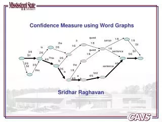
quest 1/6 a sense 1/6 the 1/6 Sil 1/6 is 2/6 1/6 guest sentence Sil 3/6 2/6 1/6 5/6 Sil This 2/6 4/6 is 3/6 4/6 3/6 the Sil sentence 2/6 this 1/6 is test a 4/6 4/6 a Confidence Measure using Word Graphs Sridhar Raghavan
Abstract • Confidence measure using word posterior: • There is a strong need for determining the confidence of a word hypothesis in a LVCSR system because conventional viterbi decoding just generates the overall one best sequence, but the performance of a speech recognition system is based on Word error rate and not sentence error rate. • Word posterior probability in a hypothesis is a good estimate of the confidence. • The word posteriors can be computed from a word graph where the links correspond to the words. • A forward-backward algorithm is used to compute the link posteriors.
Foundation The equation for computing the posterior of the word is as follows [Wessel.F]: The idea here is to sum up the posterior probabilities of all those word hypothesis sequences that contain the word ‘w’ with same start and end times.
Foundation: continued… We cannot compute the above posterior directly, so we decompose it into likelihood and priors using Baye’s rule. The value in the numerator can be computed using the well known forward backward algorithm. The denominator term is simply the sum of the numerator for all words ‘w’ occuring in the same time instant ta to te.
1/6 a sense 1/6 the 1/6 Sil 1/6 is 2/6 1/6 guest sentence Sil 3/6 2/6 1/6 5/6 Sil This 2/6 4/6 is 3/6 4/6 3/6 the Sil sentence 2/6 this 1/6 is test a 4/6 4/6 • What is exactly a word posterior from a word graph? A word posterior is a probability that is computed by considering a word’s acoustic score, language model score and its presence is a particular path through the word graph. An example of a word graph is given below, note that the nodes are the start-stop times and the links are the words. The goal is to determine the link posterior probabilities. Every link holds an acoustic score and a language model probability. quest
quest 1/6 a sense 1/6 the 1/6 Sil 1/6 is 2/6 1/6 guest sentence Sil 3/6 2/6 1/6 5/6 Sil This 2/6 4/6 is 3/6 4/6 3/6 the Sil sentence 2/6 this 1/6 is test a 4/6 4/6 a • Example Let us consider an example as shown below: The values on the links are the likelihoods.
Forward-backward algorithm Using forward-backward algorithm for determining the link probability. The equations used to compute the alphas and betas for an HMM are as follows: Computing alphas: Step 1: Initialization: In a conventional HMM forward-backward algorithm we would perform the following – We need to use a slightly modified version of the above equation for processing a word graph. The emission probability will be the acoustic score and the initial probability is taken as 1 since we always begin with a silence.
Forward-backward algorithm continue… The α for the first node in the word graph is computed as follows: Step 2: Induction This step is the main reason we use forward-backward algorithm for computing such probabilities. The alpha values computed in the previous step is used to compute the alphas for the succeeding nodes. Note: Unlike in HMMs where we move from left to right at fixed intervals of time, over here we move from one start time of a word to the next closest word’s start time.
Forward-backward algorithm continue… Let us see the computation of the alphas from node 2, the alpha for node 1 was computed in the previous step during initialization. Node 2: α=1.675E-03 α =0.5025 is 4 Node 3: α =1 3/6 2/6 Sil 1 4/6 3 3/6 3/6 Sil Node 4: this 2 α =0.5 The alpha calculation continues in this manner for all the remaining nodes The forward backward calculation on word-graphs is similar to the calculations used on HMMs, but in word graphs the transition matrix is populated by the language model probabilities and the emission probability corresponds to the acoustic score.
Forward-backward algorithm continue… Once we compute the alphas using the forward algorithm we begin the beta computation using the backward algorithm. The backward algorithm is similar to the forward algorithm, but we start from the last node and proceed from right to left. Step 1 : Initialization Step 2: Induction
Forward-backward algorithm continue… Let us see the computation of the beta values from node 14 and backwards. Node 14: β=1.66E-3 β=0.1667 1/6 sense 14 1/6 Sil 1/6 11 sentence Sil Node 13: 5/6 13 15 4/6 β=1 sentence β=0.833 12 Node 12: β=5.55E-3
Forward-backward algorithm continue… Node 11: In a similar manner we obtain the beta values for all the nodes till node 1. We can compute the probabilities on the links (between two nodes) as follows: Let us call this link probability as Γ. Therefore Γ(t-1,t) is computed as the product of α(t-1)*ß(t)*aij. These values give the un-normalized posterior probabilities of the word on the link considering all possible paths through the link.
Word graph showing the computed alphas and betas This is the word graph with every node with its corresponding alpha and beta value. α=1.675E-5 β=4.61E-9 α=2.79E-8 β=2.766E-6 α=1.2923E-13 β=0.1667 α=7.751E-11 β=1.66E-3 α=1.675E-03 β=1.536E-11 α =0.5025 β=5.740E-12 quest 1/6 a sense 14 1/6 the 1/6 Sil 8 1/6 α =1 β=2.8843E-14 is 2/6 4 1/6 guest 11 sentence Sil 3/6 2/6 1/6 5/6 Sil 6 This 2/6 1 4/6 13 15 3 is 9 4/6 3/6 α=1.861E-8 β=2.766E-6 α=2.88E-14 β=1 3/6 the Sil sentence 5 α=3.438E-12 β=0.833 2/6 this 1/6 α=3.35E-3 β=8.527E-10 is test 2 a 4/6 4/6 12 α =0.5 β=2.87E-14 7 10 α=4.964E-10 β=5.55E-3 α=7.446E-8 β=3.7E-5 α=1.117E-5 β=2.512E-7 Assumption here is that the probability of occurrence of any word is 0.01. i.e. we have 100 words in a loop grammar
Link probabilities calculated from alphas and betas The following word graph shows the links with their corresponding link posterior probabilities (not yet normalized). Γ=4.649E-13 Γ=4.649E-13 quest 1/6 Γ=7.72E-14 a sense 14 1/6 Γ=1.292E-15 the 1/6 Γ=1.292E-13 Γ=7.71E-14 Sil 8 1/6 is 2/6 Γ=5.74E-12 4 1/6 11 guest sentence Sil 3/6 2/6 1/6 5/6 6 Sil Γ=6.45E-13 This 2/6 13 1 4/6 15 3 is Γ=3.08E-13 9 Γ=1.549E-13 4/6 3/6 3/6 the Γ=3.438E-14 Sil Γ=4.288E-12 sentence 5 Γ=2.87E-14 2/6 this 1/6 Γ=3.08E-13 is test Γ=2.87E-14 2 a 4/6 Γ=4.136E-12 12 4/6 7 10 Γ=8.421E-12 Γ=4.136E-12 Γ=4.136E1-12 By choosing the links with the maximum posterior probability we can be certain that we have included most probable words in the final sequence.
Using it on a real application Using the algorithm on real application: * Need to perform word spotting without using a language model i.e. we can only use a loop grammar. * In order to spot the word of interest we will construct a loop grammar with just this one word. * Now the final one best hypothesis will consist of a sequence of the same word repeated N times. So, the challenge here is to determine which of these N words actually corresponds to the word of interest. * This is achieved by computing the link posterior probability and selecting the one with the maximum value.
1-best output from the word spotter The recognizer puts out the following output :- 0000 0023 !SENT_START -1433.434204 0023 0081 BIG -4029.476440 0081 0176 BIG -6402.677246 0176 0237 BIG -4080.437500 0237 0266 !SENT_END -1861.777344 We have to determine which of the three instances of the word actually exists.
2 -912 -1095 3 -1433 -1888 sent_start -1070 0 1 -2875 4 -1232 -4029 -1861 sent_end -6402 -4056 8 5 6 7 Lattice from one of the utterances For this example we have to spot the word “BIG” in an utterance that consists of three words (“BIG TIED GOD”). All the links in the output lattice contains the word “BIG”. The values on the links are the acoustic likelihoods in log domain. Hence a forward backward computation just involves addition of these numbers in a systematic manner.
α =-2528 β=-15533 2 -912 α =-6761 β=-14621 α =0 β=-67344 -1095 3 -1433 -1888 sent_start -1070 1 0 -2875 α =-12139 β=-13551 α =-1433 β=-65911 4 -1232 -4029 -1861 sent_end -6402 -4056 8 5 6 7 α =-18833 β=-12319 α =-25235 β=-5917 α =-29291 β=-1861 α =-31152 β=0 • Alphas and betas for the lattice The initial probability at both the nodes is ‘1’. So, its logarithmic value is 0. The language model probability of the word is also ‘1’ since it is the only word in the loop grammar.
Link posterior calculation It is observed that we can obtain a greater discrimination in confidence levels if we also multiply the final probability with the likelihood of the link other than the corresponding alphas and betas. In this example we add the likelihood since it is in log domain. 2 Γ=-18061 Γ=-18061 Γ=-67344 Γ=-17942 3 sent_start Γ=-21382 1 0 Γ=-17859 4 Γ=-25690 Γ=-17781 Γ=-31152 Γ=-31152 Γ=-31152 sent_end 8 5 6 7
Inference from the link posteriors Link 1 to 5 corresponds to the first word time instance while 5 to 6 and 6 to 7 correspond to the second and third word instances respectively. It is very clear from the link posterior values that the first instance of the word “BIG” has a much higher probability than the other two. Note: The part that is missing in this presentation is the normalization of these probabilities, this is needed to make comparison between various link posteriors.
References: • F. Wessel, R. Schlüter, K. Macherey, H. Ney. "Confidence Measures for Large Vocabulary Continuous Speech Recognition". IEEE Trans. on Speech and Audio Processing. Vol. 9, No. 3, pp. 288-298, March 2001 • Wessel, Macherey, and Schauter, "Using Word Probabilities as Confidence Measures, ICASSP'97 • G. Evermann and P.C. Woodland, “Large Vocabulary Decoding and Confidence Estimation using Word Posterior Probabilities in Proc. ICASSP 2000, pp. 2366-2369, Istanbul. • X. Huang, A. Acero, and H.W. Hon, Spoken Language Processing - A Guide to Theory, Algorithm, and System Development, Prentice Hall, ISBN: 0-13-022616-5, 2001 • J. Deller, et. al., Discrete-Time Processing of Speech Signals, MacMillan Publishing Co., ISBN: 0-7803-5386-2, 2000