Download
1 / 17
170 likes | 243 Views
Topological Neural Networks. Bear, Connors & Paradiso (2001). Neuroscience: Exploring The Brain . Pg. 474. Self-Organizing Maps. SOMs = Competitive Networks where: 1 input and 1 output layer. All input nodes feed into all output nodes.

E N D
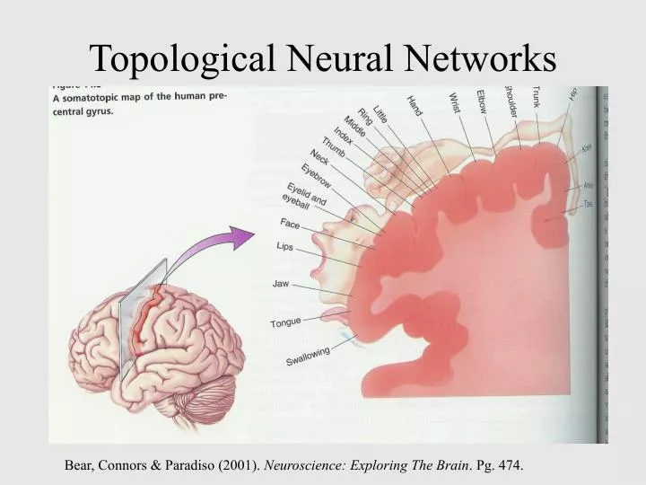
Topological Neural Networks Bear, Connors & Paradiso (2001). Neuroscience: Exploring The Brain. Pg. 474.
Self-Organizing Maps • SOMs = Competitive Networks where: • 1 input and 1 output layer. • All input nodes feed into all output nodes. • Output layer nodes are NOT a clique. Each node has a few neighbors. • On each training input, all output nodes that are within a topological distance, dT, of D from the winner node will have their incoming weights modified. • dT(yi,yj) = # nodes that must be traversed in the output layer in moving between output nodes yi and yj. • D is typically decreased as training proceeds. Output Input Partially Intraconnected Fully Interconnected
There Goes The Neighborhood D = 1 D = 2 D = 3 • As the training period progresses, gradually decrease D. • Over time, islands form in which the center represents the centroid C of a set • of input vectors, S, while nearby neighbors represent slight variations on C and • more distant neighbors are major variations. • These neighbors may only win on a few (or no) input vectors, while the island • center will win on many of the elements of S.
Self Organization • In the beginning, the Euclidian distance dE(yl,yk) and Topological distance dT(yl,yk) between output nodes yl and yk will not be related. • But during the course of training, they will become positively correlated: Neighbor nodes in the topology will have similar weight vectors, and topologically distant nodes will have very different weight vectors. Emergent Structure of Output Layer Euclidean Neighbor Topological Neighbor Before After
Self-Organized Maps for Robot Navigation Owen & Nehmzow (1998) Task: Autonomous robot navigation in a laboratory Goals: 1. Find a useful internal representation (i.e. map) that supports an intelligent choice of actions for the given sensory inputs 2. Let the robot build/learn the map itself - Saves the user from specifying it. - Allows the robot to handle new environments. - By learning the map in a noisy, real-world situation, the robot will be more apt to handle other noisy environments. Approach: • Use an SOM to organize situation-action vectors. • The emerging structure of the SOM then constitutes the robot’s functional internal representation of both the outside world and the appropriate actions to take in different regions of that world.
“Turn Right & Slow Down R 1. Record Sensory Info 2. Get correct actions 3. Input Vector = Sensory Inputs & Actions The Training Phase Input Output 5. Update Winner & Neighbors 4. Run SOM on Input Vector
R 1. Record Sensory Info A 4. Read Recommended Actions from the Winner’s Weight Vector The Testing Phase 2. Input Vector = Sensory Inputs & No Actions Input Output 3. Run SOM on Input Vector
Clustering of Perceptual Signatures • The general closeness of successive winners shows a correlation between points & distances in the objective world and the robot’s functional view of that world. • Note: A trace of the robot’s path on a map of the real world (i.e. lab floor) would have ONLY short moves. The sequence of winner nodes during the testing phase of a typical navigation task.
SOM for Navigation Summary • SOM Regions = Perceptual Landmarks = Sets of similar perceptual patterns • Navigation = Association of actions with perceptual landmarks • Behavior is controlled by the robot’s subjective functional interpretation of the world, which may abstract the world into a few key perceptual categories. • No extensive objective map of the entire environment is required. • Useful maps are user & task centered. • Robustness (Fault Tolerance): The robot also navigates successfully when a few of its sensors are damaged => The SOM has generalized from the specific training instances. • Similar neuronal organizations, with correlations between points in the visual field and neurons in a brain region, are found in many animals.
1 kHz 4 kHz 10 kHz 20 kHz Tonotopic Maps in the Auditory System Auditory Cortex Tonotopy preserved through all 7 levels of processing MGN Source Localization Via Delay Lines Inferior Colliculus Superior Olive 1 kHz Ventral Cochlear Nucleus 4 kHz 10 kHz Spiral Ganglion 20 kHz Sp. Gang. Cochlea Cochlear Nucleus Cochlea (Inner Ear)
Source Location Detection Neurons: Need 2 simultaneous inputs to fire Transformer Neurons: Convert sound frequency into a neural firing pattern, which is phase-locked to the sound waves (although lower freq). Source Localization using Delay Lines Straight Ahead! Owls have different ear heights, so they can use the same mechanism for horizontal and vertical localization Left 90o Right 90o Left 45o Right 45o Right Ear Left Ear Topological Map = Similar dirs detected by neighboring cells.
Occular Dominance & Orientation Columns Right eye Left eye Right eye Left eye Layers 5 & 6 of V1 LGN Neural Response (Firing rate) Retina • 2 Topological Maps • Cells respond to lines at particular angles, • and nearby cells respond to similar angles. • Regions of cells respond to the same eye. -90o 90o 0o Orientation Angle
Self-Organizing Maps of Orientation Columns Retina Training Patterns Visual Cortex • Each VC cell gets input from • all retinal cells. • Initially, all weights random. • Each pattern is presented, and • the ”winning” VC cell gets • to change its weights to better • match the input. • Nearby cells in a slowly- • shrinking neighborhood also • update their weights.
Emerging Orientation Preferences • Many VC cells show a strong preference for a particular orientation. • Neighboring cells show similar preferences. • Gradients of preferred orientations often form along vertical, horizontal and diagonal axes.
Biological Kohonen Maps • The orientation columns clearly emerge from a Kohonen algorithm of weight-change spreading in a slowly-shrinking neighborhood. • But this lacks biological realism. • So classic Kohonen maps cannot explain the formation of orientation columns. • However, the basic neurophysiological mechanisms of late-stage long-term potentiation (late LTP) can be used in a modified Kohonen map to produce similar orientation-columns. • Key idea: When a pre-synaptic (retinal) node R and post-synaptic (VC) node V both fire, then: • the RV weight should be increased, • R should produce more axons, some of which will spread to OTHER post-synaptic nodes, V2,V3..in the general neighborhood of V. • So each training pattern will produce a winner node, V, and portions of the input weights to V will be randomly distributed to the input weights of some neighboring VC nodes: Weight(R,V) will affect Weight(R,V2), Weight(R,V3), etc. • Extent of random neighborhoods gradually decreases (just as the degree of plasticity decreases during biological development)
Retina R Winner VC node Random neighbor Visual Cortex