Modifying Floating-Point Precision with Binary Instrumentation
Modifying Floating-Point Precision with Binary Instrumentation. Michael Lam University of Maryland, College Park Jeff Hollingsworth, Advisor. Background. Floating-point represents real numbers as (± sgnf × 2 exp ) Sign bit Exponent Significand ( “ mantissa ” or “ fraction ” )

Modifying Floating-Point Precision with Binary Instrumentation
E N D
Presentation Transcript
Modifying Floating-Point Precision with Binary Instrumentation Michael Lam University of Maryland, College Park Jeff Hollingsworth, Advisor
Background • Floating-point represents real numbers as (± sgnf × 2exp) • Sign bit • Exponent • Significand (“mantissa” or “fraction”) • Floating-point numbers have finite precision • Single-precision: 24 bits (~7 decimal digits) • Double-precision: 53 bits (~16 decimal digits) 8 4 32 0 16 IEEE Single Exponent (8 bits) Significand (23 bits) 8 4 64 32 0 16 IEEE Double Exponent (11 bits) Significand (52 bits) 2
Example 1/10 0.1 Single-precision Double-precision Images courtesy of BinaryConvert.com 3
Motivation • Finite precision causes round-off error • Compromises “ill-conditioned” calculations • Hard to detect and diagnose • Increasingly important as HPC scales • Double-precision data movement is a bottleneck • Streaming processors are faster in single-precision (~2x) • Need to balance speed (singles) and accuracy (doubles) 4
Previous Work • Traditional error analysis (Wilkinson 1964) • Forwards vs. backwards • Requires extensive numerical analysis expertise • Interval/affine arithmetic (Goubault2001) • Conservative static error bounds are largely unhelpful High bound Value Correct value Low bound Time 5
Previous Work • Manual mixed-precision (Dongarra 2008) • Requires numerical expertise • Fallback: ad-hoc experiments • Tedious, time-consuming, and error-prone 1: LU ← PA 2: solve Ly = Pb 3: solve Ux0 = y 4: for k = 1, 2, ... do 5: rk ← b – Axk-1 6: solve Ly = Prk 7: solve Uzk = y 8: xk ← xk-1 + zk 9: check for convergence 10: end for Mixed-precision linear solver algorithm Red text indicates steps performed in double-precision (all other steps are single-precision) 6
Our Goal Develop automated analysis techniques to inform developers about floating-point behavior and make recommendations regarding the precision level that each part of a computer program must use in order to maintain overall accuracy. 7
Framework CRAFT: Configurable Runtime Analysis for Floating-point Tuning • Static binary instrumentation • Controlled by configuration settings • Replace floating-point instructions with new code • Re-write a modified binary • Dynamic analysis • Run modified program on representative data set • Produces results and recommendations 8
Advantages • Automated • Minimize developer effort • Ensure consistency and correctness • Binary-level • Include shared libraries without source code • Include compiler optimizations • Runtime • Dataset and communication sensitivity 9
Implementation • Current approach: in-place replacement • Narrowed focus: doubles singles • In-place downcast conversion • Flag in the high bits to indicate replacement 8 4 64 32 0 16 Double downcast conversion 8 4 64 32 0 16 Replaced Double 7 F F 4 D E A D Non-signalling NaN 8 4 32 0 16 Single 10
Example gvec[i,j] = gvec[i,j] * lvec[3] + gvar 1 movsd0x601e38(%rax, %rbx, 8) %xmm0 2 mulsd-0x78(%rsp) %xmm0 3 addsd-0x4f02(%rip) %xmm0 4 movsd %xmm0 0x601e38(%rax, %rbx, 8) 11
Example gvec[i,j] = gvec[i,j] * lvec[3] + gvar 1 movsd0x601e38(%rax, %rbx, 8) %xmm0 check/replace -0x78(%rsp) and %xmm0 2 mulss-0x78(%rsp) %xmm0 check/replace -0x4f02(%rip) and %xmm0 3 addss-0x20dd43(%rip) %xmm0 4 movsd %xmm0 0x601e38(%rax, %rbx, 8) 12
Implementation original instruction in block block splits double single conversion initialization cleanup 13
Autoconfiguration • Helper script • Generates and tests a variety of configurations • Keeps a “work queue” of untested configurations • Brute-force attempt to find maximal replacement • Algorithm: • Initially, build individual configurations for each function and add them to the work queue • Retrieve the next available configuration and test it • If it passes, add it to the final configuration • If it fails, build individual configurations for any child members (basic blocks, instructions) and add them to the queue • Build and test the final configuration 15
NAS Benchmarks • EP (Embarrassingly Parallel) • Generate independent Gaussian random variates using the Marsaglia polar method • CG (Conjugate gradient) • Estimate the smallest eigenvalue of a matrix using the inverse iteration with the conjugate gradient method • FT (Fourier Transform) • Solve a three-dimensional partial differential equation (PDE) using the fast Fourier transform (FFT) • MG (MultiGrid) • Approximate the solution to a three-dimensional discrete Poisson equation using the V-cycle multigrid method 16
Results Results shown for final configuration only. All benchmarks were 8-core versions compiled by the Intel Fortran compiler with optimization enabled. Tests were performed on the Sierra cluster at LLNL (Intel Xeon 2.8GHz w/ twelve cores and 24 GB memory per node running 64-bit Linux). 17
Observations • randlc / vranlc • Random number generators are dependent on a 64-bit floating-point data type • Accumulators • Multiple operations concluded with an addition • Requires double-precision only for the final addition • Minimal dataset-based variation • Larger variation due to optimization level 18
Future Work Automated configuration tuning 19
Conclusion Automated instrumentation techniques can be used to implement mixed-precision configurations for floating-point code, and there is much opportunity in the future for automated precision recommendations. 20
Acknowledgements Jeff Hollingsworth, University of Maryland (Advisor) Drew Bernat, University of Wisconsin Bronis de Supinski, LLNL Barry Rountree, LLNL Matt Legendre, LLNL Greg Lee, LLNL Dong Ahn, LLNL http://sourceforge.net/projects/crafthpc/ 21