Download
1 / 36
370 likes | 494 Views
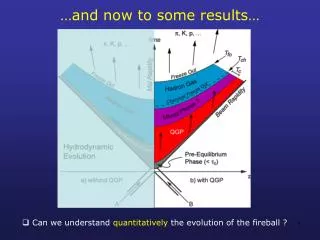
…and now to some results…. Can we understand quantitatively the evolution of the fireball ? . Chemical composition of the fireball. It is extremely interesting to measure the multiplicity of the various particles produced in the collision chemical composition.

E N D
…and now to some results… • Can we understand quantitatively the evolution of the fireball ?
Chemical composition ofthe fireball • It is extremely interesting to measure the multiplicity of the various • particles produced in the collision chemical composition • The chemical composition of the fireball is sensitive to • Degree of equilibrium of the fireball at (chemical) freeze-out • Temperature Tchat chemical freeze-out • Baryonic content of the fireball • This information is obtained through the use of statistical models • Thermal and chemical equilibrium at chemical freeze-out assumed • Write partition function and use statistical mechanics • (grand-canonical ensemble) assume hadron production is a • statistical process • System described as an ideal gas of hadrons and resonances • Follows original ideas by Fermi (1950s) and Hagedorn (1960s)
Hadron multiplicities vss • Baryons from colliding • nuclei dominate at low s • (stopping vs transparency) • Pions are the most • abundant mesons (low • mass and production • threshold) • Isospin effects at low s • pbar/p tends to 1 at • high s • K+ and more produced • than their anti-particles • (light quarks present in • colliding nuclei)
Statistical models • In statistical models of hadronization • Hadron and resonance gas with baryons and mesons • having m 2 GeV/c2 • Well known hadronic spectrum • Well known decay chains • These models have in principle 5 free parameters: • T : temperature • mB : baryochemical potential • mS : strangeness chemical potential • mI3 : isospin chemical potential • V : fireball volume • But three relations based on the knowledge of the initial state • (NS neutrons and ZS “stopped” protons) allow us to reduce the • number of free parameters to 2 Only 2 free parameters remain: T and mB
Particle ratios at AGS • Results on ratios: cancel a significant fraction of systematic uncertainties • AuAu - Ebeam=10.7 GeV/nucleon - s=4.85 GeV • Minimum c2 for: T=124±3 MeV mB=537±10 MeV c2 contour lines
Particle ratios at SPS • PbPb - Ebeam=40 GeV/ nucleon - s=8.77 GeV • Minimum c2 for: T=156±3 MeV mB=403±18 MeV c2 contour lines
Particle ratios at RHIC • AuAu - s=130 GeV • Valore minimo di c2 per: T=166±5 MeV mB=38±11 MeV c2 contour lines
Thermal model parameters vs. s • The temperature Tch quickly • increases with s up to ~170 MeV • (close to critical temperature for the • phase transition!) at s ~ 7-8 GeV • and then stays constant • The chemical potential B decreases • with s in all the energy range • explored from AGS to RHIC
Chemical freeze-out and phase diagram • Compare the evolution vss of the (T,B) pairs with the QCD phase • diagram • The points approach the phase transition region already at SPS energy • The hadronic system reaches chemical equilibrium immediately after • the transition QGPhadronstakes place
News from LHC • Thermal model fits for yields • and particle ratios • T=164 MeV, excluding protons • Unexpected results for protons: abundances below thermal model • predictions work in progress to understand this new feature!
Chemical freeze-out • Fits to particle abundances • or particle ratios in • thermal models • These models assume • chemical and thermal • equilibrium and describe • very well the data • The chemical freeze-out • temperature saturates • at around 170 MeV, while • B approaches zero at • high energy • New LHC data still • challenging
Collective motion in heavy-ion collisions (FLOW) Radial flow connection with thermal freeze-out Elliptic flow connection with thermalization of the system Let’s start from pT distributions in pp and AA collisions
pTdistributions • Transverse momentum distributions of produced particles can provide important information on the system created in the collisions • Low pT(<~1 GeV/c) • Soft production • mechanisms • 1/pTdN/dpT ~exponential, • Boltzmann-like and almost • independent on s • High pT (>>1 GeV/c) • Hard production • mechanisms • Deviation from exponential • behaviour towards • power-law
Let’s concentrate on low pT • In pp collisions at low pT • Exponential behaviour, identical for • all hadrons (mTscaling) • Tslope~ 167 MeV for all particles • These distribution look like thermal spectra and Tslope can be seen as • the temperature corresponding to the emission of the particles, when • interactions between particles stop (freeze-out temperature, Tfo) 14
pTand mTspectra • Slightly different shape of spectra, • when plotted as a function of pTor mT Evolution of pT spectra vsTslope, higher T implies “flatter” spectra
Breaking of mT scaling in AA • Harder spectra (i.e. larger Tslope) • for larger mass particles • Consistent with a shift towards • larger pTof heavier particles
Breaking of mT scaling in AA • Tslopedepends linearly • on particle mass • Interpretation: • there is a collective • motion of all particles • in the transverse plane • with velocity v, • superimposed to • thermal motion, • which gives Such a collective transverse expansion is called radial flow (also known as “Little Bang”!)
y v x v Flow in heavy-ion collisions • Flow: collective motion of particles superimposed to thermal motion • Due to the high pressures generated when nuclear matter is heated • and compressed • Flux velocity of an element of the system is given by the sum of the • velocities of the particles in that element • Collective flow is a correlation between the velocity v of a volume • element and its space-time position
Radial flow at SPS y x • Radial flow breaks mT • scaling at low pT • With a fit to identified • particle spectra one can • separate thermal and • collective components • At top SPS energy • (s=17 GeV): • Tfo= 120 MeV • = 0.50 19
Radial flow at RHIC y x • Radial flow breaks mT • scaling at low pT • With a fit to identified • particle spectra one can • separate thermal and • collective components • At RHIC energy • (s=200 GeV): • Tfo~ 100 MeV • ~ 0.6 20
Radial flow at LHC • Pion, proton and kaon spectra • for central events (0-5%) • LHC spectra are harder than • those measured at RHIC • Tfo= 95 10 MeV • = 0.65 0.02 Clear increase of radial flow at LHC, compared to RHIC (same centrality) 21
Thermal freeze-out • Fits to pT spectra allow • us to extract the • temperature Tfoand the • radial expansion velocity • at the thermal freeze-out • The fireball created in • heavy-ion collisions • crosses thermal • freeze-out at 90-130 • MeV, depending on • centrality and s • At thermal freeze-out the • fireball has a collective • radial expansion, with a • velocity 0.5-0.7 c
y YRP x Anisotropic transverse flow • In heavy-ion collisions the impact parameter creates a “preferred” • direction in the transverse plane • The “reaction plane” is the plane defined by the impact parameter and • the beam direction 23
y z x Anisotropic transverse flow • In collisions with b 0 (non central) the fireball has a geometric • anisotropy, with the overlap region being an ellipsoid • Macroscopically (hydrodynamic description) • The pressure gradients, i.e. the forces “pushing” the particles are • anisotropic (-dependent), and larger in the x-z plane • -dependent velocity anisotropic azimuthal distribution of particles • Microscopically • Interactions between produced • particles (if strong enough!) can • convert theinitial geometric • anisotropy in an anisotropy in • the momentum distributions • of particles, which can be • measured Reaction plane
Anisotropic transverse flow • Starting from the azimuthal distributions of the produced particles with • respect to the reaction plane RP, one can use a Fourier decomposition • and write • The terms in sin(-RP) are not present since the particle distributions • need to be symmetric with respect to RP • The coefficients of the various harmonics describe the deviations with • respect to an isotropic distribution • From the properties of Fourier’s series one has
v2 coefficient: elliptic flow Elliptic flow • v2 0 means that there is a • difference between the • number of particles directed • parallel (00 and 1800) and • perpendicular (900 and 2700) • to the impact parameter • It is the effect that one may • expect from a difference of • pressure gradients parallel • and orthogonal to the impact • parameter IN PLANE OUT OF PLANE v2 > 0 in-plane flow, v2 < 0 out-of-plane flow
Elliptic flow - characteristics • The geometrical anisotropy which • gives rise to the elliptic flow • becomes weaker with the evolution • of the system • Pressure gradients are stronger in • the first stages of the collision • Elliptic flow is therefore an observable • particularly sensitive to the first stages • (QGP)
Elliptic flow - characteristics • The geometric anisotropy (X= elliptic deformation of the fireball) • decreases with time • The momentum anisotropy (p , which is the real observable), according • to hydrodynamic models: • grows quickly in the QGP state ( < 2-3 fm/c) • remains constant during the phase transition (2<<5 fm/c), which in • the models is assumed to be first-order • Increases slightly in the hadronic phase ( > 5 fm/c)
Results on elliptic flow: RHIC • Elliptic flow depends on • Eccentricity of the overlap region, which decreases for central events • Number of interactions suffered by particles, which increases for • central events • Very peripheral collisions: • large eccentricity • few re-interactions • small v2 • Semi-peripheral collisions: • large eccentricity • several re-interactions • largev2 • Semi-central collisions: • no eccentricity • many re-interactions • v2 small (=0 for b=0) 29
Hydrodynamic limit STAR PHOBOS RQMD v2vs centrality at RHIC • Measured v2 values are in good agreement with ideal hydrodynamics • (no viscosity) for central and semi-central collisions, using parameters • (e.g. fo) extracted from pT spectra • Models, such as RQMD, based on a hadronic cascade, do not • reproduce the observed elliptic flow, which is therefore likely • to come from a partonic(i.e. deconfined) phase
Hydrodynamic limit STAR PHOBOS RQMD v2vs centrality at RHIC • Interpretation • In semi-central collisions there is a fast thermalization and the • produced system is an ideal fluid • When collisions become peripheral thermalization is incomplete • or slower • Hydro limit corresponds to a perfect fluid, the effect of viscosity is • to reduce the elliptic flow
v2 vs transverse momentum • At low pThydrodynamics reproduces data • At high pT significant deviations are observed • Natural explanation: high-pTparticles quickly escape the fireball • without enough rescattering no thermalization, hydrodynamics • not applicable
v2vspTfor identified particles • Hydrodynamics can reproduce rather well also the dependence of • v2 on particle mass, at low pT
Elliptic flow, from RHIC to LHC • Elliptic flow, integrated over pT, increases by 30% from RHIC to LHC In-plane v2 (>0) for very low √s: projectile and target form a rotating system In-plane v2 (>0) at relativistic energies (AGS and above) driven by pressure gradients (collective hydrodynamics) Out-of-plane v2 (<0) for low √s, due to absorption by spectator nucleons
Elliptic flow at LHC • The difference in the pT • dependence of v2 between • kaons, protons and pions (mass • splitting) is larger at LHC • v2 as a function of pTdoes not • change between RHIC and LHC • The 30% increase of integrated • elliptic flow is then due to the • larger pT at LHC coming from • the larger radial flow • This is another consequence of • the larger radial flow which • pushes protons (comparatively) • to larger pT
Conclusions on elliptic flow • In heavy-ion collisions at RHIC and LHC one observes • Strong elliptic flow • Hydrodynamic evolution of an ideal fluid (including a QGP phase) • reproduces the observed values of the elliptic flow and their • dependence on the particle masses • Main characteristics • Fireball quickly reaches thermal equilibrium (equ~ 0.6 – 1 fm/c) • The system behaves as a perfect fluid (viscosity ~0) • Increase of the elliptic flow at LHC by ~30%, mainly due to larger • transverse momenta of the particles