Physical and Mathematical Basics of Stellar Dynamics (best textbook: Binney and Tremaine 1997)

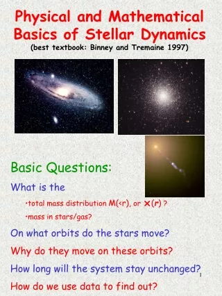
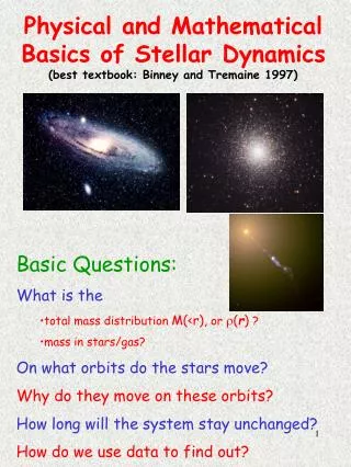
1. Physical and Mathematical Basics of Stellar Dynamics(best textbook: Binney and Tremaine 1997) • Basic Questions: • What is the • total mass distribution M(<r), or r(r) ? • mass in stars/gas? • On what orbits do the stars move? • Why do they move on these orbits? • How long will the system stay unchanged? • How do we use data to find out?

2. Collisionless vs. Collisional Matter How often do stars in a galaxy collide? - ignore binary stars - order of magnitude estimates • RSun 7x1010 cm; DSun-Cen  1019 cm! => collisions extremely unlikely! …and in galaxy centers? Mean surface brightness of the Sun is  = - 11mag/sqasec, which is distance independent. The central parts of other galaxies have ~ 12 mag/sqasec. Therefore, (1 - 10-9) of the projected area is empty. • Even near galaxy centers, the path ahead of stars is empty.

3. Dynamical time-scale (=typical orbital period) Milky Way: R~8kpc v~200km/s torb~240 Myrs  torb~tHubble/50 Stars in a galaxy feel the gravitational force of other stars. But of which ones? • consider homogeneous distribution of stars, and force exerted on one star by other stars seen in a direction d within a slice of [r,rx(1+e)] • => dF ~ GdM/r2 = Gρ xr(!)xdΩ • - gravity from the multitude of distant stars dominates!

4. What about (diffuse) interstellar gas? • continuous mass distribution • gas has the ability to loose (internal) energy through radiation. • Two basic regimes for gas in a potential well of ‚typical orbital velocity‘, v • • kT/m  v2  hydrostatic equilibrium • • kT/m << v2, as for atomic gas in galaxies • in the second case: • • supersonic collisions  shocks  (mechanical) heating  (radiative) cooling  energy loss • • for a given (total) angular momentum, what‘s the minimum energy orbit? A (set of) concentric (co-planar), circular orbits. • => cooling gas makes disks!

5. Dynamics of Collisionless Matter: (see Appendix) Phase space: dx, dv We describe a many-particle system by its distribution functionf(x,v,t) = density of stars (particles) within a phase space element Starting point: Boltzmann Equation(= phase space continuity equation) It says: if I follow a particle on its gravitational path (=Lagrangian derivative) through phase space, it will always be there. A rather ugly partial differential equation! Note: we have substituted gravitational force for accelaration! To simplify it, one takesvelocity moments: i.e. n = 0,1, ... on both sides

6. Moments of the Boltzmann Equation mass conservation Oth Moment 1st Moment “Jeans Equation” The three terms can be interpreted as: momentum change pressure force grav. force r: mass density; v/u: indiv/mean particle velocity

7. Let‘s look for some familiar ground ... If has the simple isotropic form as for an „ideal gas“ and if the system is in steady state , then we get simple hydrostatic equilibrium Before getting serious about solving the „Jeans Equation“, let‘s play the integration trick one more time ...

8. Virial Theorem To keep the math simple, we consider the one-dimensional analog of I.4 in steady state: I.5 „velocity dispersion“ After integrating over velocities, let‘sintegrate over : [one needs to use Gauss’ theorem etc..]

9. Application of the Virial Theorem • Ekin ~ ½ M<v2>,butEpot ~ GM2<1/R> • can estimate Mass M~<v2>R/G What observables do we need? • characteristic “virial” radius • characteristic velocities of the particles Practical problem: Observables • Projected distances • Line-of-sight velocities Examples: • Globular cluster • R~5pc, s~5km/s  M=3x104 Msun • Elliptical Galaxy • R~3kpc, s~200km/s  M=3x1010 Msun

10. Application of the Jeans Equation • Goal: • Avoid “picking”right virial radius. • Account for spatial variations • Get more information than “total mass” • Simplest case • spherical: static:  • at any point can be diagonalized t: tangential velocity dispersion

11. With vector calculus ….  Jeans Equation spherical coordinates Note: (there are 2 t components) centrifugal equilibrium For a system that is locally isotropic, , II.2 becomes

12. Note: Isotropy is a mathematical assumption here, not justified by physics! Remember: is the mass density of particles under consideration (e.g. stars), while  just describes the gravitational potential acting on them. • How are  and  related? Two options: 1. „self-consistent problem“ 2. with other = dark matter + gas + ... Black Hole

13. We often have two goals in mind: a. discriminate between 1. and 2.; do we „need“ other b. Constrain total on the basis of the spatial distribution and motions of the particles described by  • Estimating from the observed kinematics for an isotropic system: II.4

14. This relation relates the total mass profile M(<r), to the observable properties of the tracers, (r) and (r)! Note: • often the density gradient () is much steeper than the dispersion gradient (): Example:

15. NGC 4374: Haering&Rix 2003 Surface Brightness Stellar Velocity Dispersion Goal:estimate the stellar/total mass within a certain radius from the light profile and the kinematics of the stars in, say, a nearby elliptical galaxy Observables: Dynamical ModellingA Simple Example

16. Modelling Scheme + Bulge radius

17. Galaxies out of Equilibrium I. Mergers and Interaction Brief History: • Zwicky and Arp (1950s and 1960s) studied “peculiar galaxies” which exhibit distortions, bridges between pairs, etc. (“Atlas of Peculiar Galaxies”, Arp 1966). • In 1956 Zwicky speculated that “tidal interactions” may cause these features.

18. In 1972, Alan and Juri Toomre published the first “realistic” simulations of galaxy interactions, matching M 51 and the “Antennae”. This paper contains two predictions: • encounters transfer orbital into internal energy  merger  spirals  “messy” ellipticalsFirst proposed mechanism of galaxy evolution! • at earlier epochs densities were higher more interactions/mergers

19. The Mechanics of Galaxy Interactions • Interactions/mergers wouldn‘t be important if galaxies are randomly dist. • ; • “capture cross section” • To get galaxy clumping (correlations) and mergers, we need dark matter (= more grav. force) To study interactions/mergers we have to solve the time-dependent Boltzmann equation:  numerical solution

20. Step 1: Create Monte-Carlo representation of and force • ;(usually ) • interpret as a probability of drawingNote: often

21. becomes# i.e. we must replace by softening to avoid 2-body interactions, becauseNsimul. Ntrue!Usually,

22. Step 2: Force Calculation • to make this Monte-Carlo calculation more accurate: N increase, m decrease, but terms in R.H.S. of # increase as N² need clever ways to evaluate the force! A. Field Expansion Approximate by (e.g. a spherical harmonics) series from where we‘ve solved ahead of time! Advantage: calculating Akis 0(N) Disadvantage: need stable geometry to pick expansion that converges quickly

23. B. Hierarchical Force Evaluation: “Tree Codes” Idea: force due to mass of size l at a distance regardless of mass distribution. Within the cell, as long as d  l. “Building” cells is an 0(N logN) process. Fig. Step 3: Find a self-consistent initial condition that is stable, e.g. bulge + disk + halo for a spiral galaxy

24. Results of Numerical Merger Simulations Much of the work has focussed on merging equal/comparably sized disk galaxies • rinit rperi parabolic orbit • parameters to characterize an encounter:  it‘s hard to do a survey of all possible encounters!

25. Basic Merging Sequence: first encounter gross distortions, tidal tails, bars (!)  rapid subsequent merger 1. Given enough observational data and simulations, it is possible to reconstruct encounters near their first peri-center passageFig. The Antennae (NGC 4038/9)

26. Fig. The Mice (NGC 4676)

27. Fig. The Whirlpool (M 51) and NGC 5195 Interesting conundrum: if merging galaxies have  ~ r-2 D.M. halos, tidal tails are not flung far enough (Mihos 1997)

28. Fig. Typical Merger Sequence

29. Tidal Drag: Why do encounters lead to mergers? Two analytic limits: a) “fast encounter”: vencounter ~vinternal in M1‘s frame internal heating of M1 b) “Dynamical Friction”: • one heavy object of mass M is moving through a sea of N objects m withN · m >> M and m << M • in scatterings:light particle gains, heavy particle looses energywith

30.  angular momentum and energy are transferred “outward” Fig.

31. Violent Relaxation (Lynden-Bell 1967) Scattering of particles off the fluctuating grav. Potential  along the orbit Fig. Note: the energy ordering of particles is preserved in a merger  population gradients are preserved!

32. Is there a “most probable” end-state for f, subject to No, not for finite mass. Also, in practice the merger ends before violent relaxation is complete. Merger Products Scales: Imagine parabolic merger of identical systems of mass Mi and binding energy Ei Mfin = 2 Mi ; Efin = 2 Ei + virial theorem

33. and  mergers make galaxies fluffier (in total!) Radial Profiles: Remnant profiles resemble r1/4 laws with  ~ r-4 at large radii, where: and if N(E)  const., then Fig.

34. Shapes and Kinematics Axis ratios and rotational support of merger products roughly resemble the population of luminous ellipticals Fig.

35. Merger Summary • Galaxy mergers do happen and will transform galaxies. • Orbital energy  internal energy • Stars (and dark matter) can be simulated quite well • merger results look much like ellipticals Intense gas inflow can and will happen (hard to quantify through simulations)

37. Appendix I: • Dynamics of CollisionlessMatter Phase space: dx, dvand itsdistribution function f(x,v,t) = density of stars (particles) within a phase space element Let‘s start with the Boltzmann Equation(= phase space continuity equation) for any set of particles (self-gravitating or not!). It says: if I follow a particle on its gravitational path (=Lagrangian derivative) through phase space, it will always be there. I.1 A rather ugly P.D.E.! So, let‘s try to take velocity moments in order to simplify it: i.e. n = 0,1, ... on both sides

38. Here we need Gauß‘ theorem I.2 A. 0th Moment I.1 with from I.2 Now, define the mass density , and the mean velocity . Then we obtain I.3 mass continuity equation

39. B. 1st Moment I.1  Note: no index summation! Now define „stress“ or „pressure“ What about the last term? with (s. I.2) and

40. All this results in the 1st Moment Equation, I.4 the so-called „Jeans Equation“ The three terms can be interpreted as: momentum change pressure force grav. force

41. Notes: is formally a „stress tensor“ is the tensor productPoints to ponder: • If particles have no individual interactions, how can there be „stress“ or „pressure“? • In this equation all interactions appear to be local, while stars actually move on „non-local“ orbit! [Remember: this equation does not describe orbits or particles, but their statistics!] • I.3: to calculate we‘d need to know • I.4: to calculate we‘d need to know , etc. The hierarchy of equations is not closed!

42. Let‘s look for some familiar ground ... If has the simple isotropic form as for an „ideal gas“ and if the system is in steady state , then we get simple hydrostatic equilibrium Before getting serious about solving the „Jeans Equation“, let‘s play the integration trick one more time ...

43. Appendix IIVirial Theorem To keep the math simple, we consider the one-dimensional analog of I.4 in steady state: I.5 „velocity dispersion“ After integrating over velocities, let‘sintegrate over : on I.5

44. Let‘s look at the terms: for finite mass r.h.s. r.h.s. From I.5 I.6

45. Application of the Virial Theorem Ekin ~ Mass, but Epot ~ Mass2  can estimate Mass How can one estimate Ekin and Epot from the observables: vi(line-of-sight) and Ri(projec-ted) of a „tracer population“, which may or may not dominate. Assumption #1: Since , we need to assume the functional form of (x), e.g. for a globular cluster of stars: I.7

46. Assumption #2: We see the system from a random direction and see the tracers at random phases in their orbit. • We use this for , because Assumption #3: System is in steady state for all macroscopic quantities.

47. If mi = const = m, we can proceed from 1.7: With , we get I.8 where R is the projected separation of par-ticles. Problem #1: If some mi are much larger the estimate is statistically insufficient!  number weighting

48. Problem #2: Random orbital phases? Tracers may extend beyond field of observation at the apocenter, or too crowded at the center. Problem #3: But we have a finite number of particles; so, what‘s the uncertainty, or variance, in this estimate? and  the relation between and has infinite variance!

49. Appendix III:Mass Density Distribution Gravitational Potential B. Newton‘s theorem (for spherical systems) 1. The gravitational potential inside a spherical shell is constant  no force. 2. The potential at a distance D from the center of a spherical shell of radius R (R < D) of mass M is  For all spherical mass distributions It is often convenient to describe a spherical potential by its circular speed (or “rotation”) curve

50. So, what‘s the gravitational potential? At the center with r  R. For an arbitrary (r), i.e. nested shells: III.4