The Structural Singularity Removal Algorithm by Pantelides
220 likes | 239 Views
Learn a systematic procedure to remove structural singularities from a model using the Algorithm of Pantelides, a symbolic index-reduction algorithm. Understand the concept through examples and equations.

The Structural Singularity Removal Algorithm by Pantelides
E N D
Presentation Transcript
This lecture deals with a procedure that can be used to remove structural singularities from a model in a systematic and algorithmic fashion. It is called the Algorithm of Pantelides. The algorithm of Pantelides is a symbolic index-reduction algorithm. The Structural Singularity Removal Algorithm by Pantelides
Structural singularities and the structure digraph Pantelides algorithm Table of Contents
I I I 1 2 3 i i C R i i L1 L2 v v v v 3 1 2 0 Structural Singularities: An Example I We compose a model using the currents, the Voltages and the potentials. Consequently, the mesh equations are being ignored. We have 7 circuit components plus the ground, therefore 27 + 1 = 15 equations. In addition, there are 4 nodes giving rise to another 3 equations. Therefore, we expect 18 equations in 18 unknowns. For passive components, it is customary to normalize the Voltages in the same direction as the currents. For active components (sources), the reverse is true.
1: I1 = f1(t) 2: I2 = f2(t) 3: I3 = f3(t) 4: uR = R · iR 5: uL1 = L1 · diL1 /dt 6: uL2 = L2 · diL2 /dt 7: iC = C · duC /dt 8: v0 = 0 9:u1 = v0 – v1 10:u2 = v3 – v2 11:u3 = v0 – v1 12:uR = v3 – v0 13:uL1 = v2 – v0 14:uL2 = v1 – v3 15:uC = v1 – v2 01 02 03 04 05 u2 07 06 09 10 11 12 13 14 08 15 u3 17 diL1 /dt I1 I2 I3 uR iR uL1 18 16 uL2 iC duC /dt v0 v1 v2 v3 u1 diL2 /dt 16: iC = iL1 + I2 17: iR = iL2 + I2 18: I1 + iC + iL2 + I3 = 0 Structural Singularities: An Example II
04 03 02 01 1:I1 = f1(t) 2:I2 = f2(t) 3:I3 = f3(t) 4: uR = R · iR 5: uL1 = L1 · diL1 /dt 6:uL2 = L2 · diL2 /dt 7:iC = C · duC /dt 8:v0 = 0 9:u1 = v0 – v1 10:u2 = v3 – v2 11:u3 = v0 – v1 12:uR = v3 – v0 13:uL1 = v2 – v0 14:uL2 = v1 – v3 15:uC = v1 – v2 03 04 05 06 07 I1 08 12 11 02 13 14 15 16 09 10 17 01 I3 uR iR uL1 diL1 /dt 18 diL2 /dt iC v1 uL2 I2 v2 v3 u1 u2 u3 duC /dt v0 16: iC = iL1 + I2 17: iR = iL2 + I2 18:I1 + iC + iL2 + I3 = 0 16 15 17 13 14 18 Structural Singularities: An Example III
04 03 02 01 1:I1 = f1(t) 2:I2 = f2(t) 3:I3 = f3(t) 4: uR = R · iR 5: uL1 = L1 · diL1 /dt 6:uL2 = L2 · diL2 /dt 7:iC = C · duC /dt 8:v0 = 0 9:u1 = v0 – v1 10:u2 = v3 – v2 11:u3 = v0 – v1 12:uR = v3 – v0 13:uL1 = v2 – v0 14:uL2 = v1 – v3 15:uC = v1 – v2 03 04 05 18 07 08 09 12 11 01 13 14 15 16 10 06 17 02 I1 uR iR uL1 I3 uL2 diL2 /dt iC duC /dt diL1 /dt v1 I2 v3 u1 u2 u3 v2 v0 16:iC = iL1 + I2 17: iR = iL2 + I2 18:I1 + iC + iL2 + I3 = 0 05 14 18 17 16 15 13 Constraint Equation All connections are blue Structural Singularities: An Example IV
The algorithm for coloring the structure digraph is completely analogous to the previously used method for making the equations causal. An implementation of the method by means of a computer program probably prefers the digraph, since this algorithm can directly be mapped onto data structures of conventional programming languages. For the human eye, the coloring of the equations may be more readable. For this reason, we shall continue, in the lecture, to color equations rather than digraphs. The vertical sorting can happen simultaneously by renumbering of the equations. Coloring of the Structure Digraph
As soon as a constraint equation has been found, this equation must be differentiated. In the algorithm of Pantelides, the differentiated constraint equation is added to the set of equations. Consequently, the set of equations has now one equation too many. In order to re-equalize the number of equations and unknowns, one of the integrators that is associated with the constraint equation is being eliminated. The Algorithm by Pantelides I
x x dx dx dt dt unknown unknown unknown known, since this is a state variable dx x unknown unknown The Algorithm by Pantelides II An additional unknown was created by the elimination of the integrator. x and dx are now algebraic variables, for which there must be found equations.
When differentiating constraint equations, it can happen that additional new variables are being created, e.g. vdv, where v is an algebraic variable. Since v was already blue (otherwise, this would not have been a constraint equation), there already exists another equation to compute v. This equation must also be differentiated. The differentiation of additional equations continues until no additional variables are being created. The Algorithm by Pantelides III
eliminated integrator dI1 + diC + diL2 + dI3 = 0 newly introduced variables The Algorithm by Pantelides : An Example I 1:I1 = f1(t) 2:I2 = f2(t) 3:I3 = f3(t) 4: uR = R · iR 5: uL1 = L1 · diL1 /dt 6:uL2 = L2 · diL2 /dt 7:iC = C · duC /dt 8:v0 = 0 9:u1 = v0 – v1 10:u2 = v3 – v2 11:u3 = v0 – v1 12:uR = v3 – v0 13:uL1 = v2 – v0 14:uL2 = v1 – v3 15:uC = v1 – v2 16:iC = iL1 + I2 17: iR = iL2 + I2 18:I1 + iC + iL2 + I3 = 0
1:I1 = f1(t) 2:I2 = f2(t) 3:I3 = f3(t) 4: uR = R · iR 5: uL1 = L1 · diL1 /dt 6:uL2 = L2 · diL2 /dt 7:iC = C · duC /dt 8:v0 = 0 9:u1 = v0 – v1 10:u2 = v3 – v2 11:u3 = v0 – v1 12:uR = v3 – v0 13:uL1 = v2 – v0 14:uL2 = v1 – v3 15:uC = v1 – v2 16:iC = iL1 + I2 17: iR = iL2 + I2 18:I1 + iC + iL2 + I3 = 0 19: dI1 + diC + diL2 + dI3 = 0 The Algorithm by Pantelides : An Example II 1:I1 = f1(t) 2:I2 = f2(t) 3:I3 = f3(t) 4: uR = R · iR 5: uL1 = L1 · diL1 /dt 6: uL2 = L2 · diL2 7:iC = C · duC /dt 8:v0 = 0 9:u1 = v0 – v1 10:u2 = v3 – v2 11:u3 = v0 – v1 12:uR = v3 – v0 13:uL1 = v2 – v0 14:uL2 = v1 – v3 15:uC = v1 – v2 16:iC = iL1 + I2 17: iR = iL2 + I2 18:I1 + iC + iL2 + I3 = 0 19: dI1 + diC + diL2 + dI3 = 0
20: dI1 = df1(t)/dt 21: dI3 = df3(t)/dt 22: diC = diL1 /dt + dI2 uL1 = L1 · diL1 /dt 23: dI2 = df2(t)/dt newly introduced variable The Algorithm by Pantelides : An Example III 1:I1 = f1(t) 2:I2 = f2(t) 3:I3 = f3(t) 4: uR = R · iR 5: uL1 = L1 · diL1 /dt 6: uL2 = L2 · diL2 7:iC = C · duC /dt 8:v0 = 0 9:u1 = v0 – v1 10:u2 = v3 – v2 11:u3 = v0 – v1 12:uR = v3 – v0 13:uL1 = v2 – v0 14:uL2 = v1 – v3 15:uC = v1 – v2 16:iC = iL1 + I2 17: iR = iL2 + I2 18:I1 + iC + iL2 + I3 = 0 19: dI1 + diC + diL2 + dI3 = 0
1:I1 = f1(t) 2:I2 = f2(t) 3:I3 = f3(t) 4: uR = R · iR 5: uL1 = L1 · diL1 /dt 6: uL2 = L2 · diL2 7:iC = C · duC /dt 8:v0 = 0 9:u1 = v0 – v1 10:u2 = v3 – v2 11:u3 = v0 – v1 12:uR = v3 – v0 13:uL1 = v2 – v0 14:uL2 = v1 – v3 15:uC = v1 – v2 16:iC = iL1 + I2 17: iR = iL2 + I2 18:I1 + iC + iL2 + I3 = 0 19: dI1 + diC + diL2 + dI3 = 0 20: dI1 = df1(t)/dt 21: dI3 = df3(t)/dt 22: diC = diL1 /dt + dI2 23: dI2 = df2(t)/dt The Algorithm by Pantelides : An Example IV
1:I1 = f1(t) 2:I2 = f2(t) 3:I3 = f3(t) 4: uR = R · iR 5: uL1 = L1 · diL1 /dt 6: uL2 = L2 · diL2 7:iC = C · duC /dt 8:v0 = 0 9:u1 = v0 – v1 10:u2 = v3 – v2 11:u3 = v0 – v1 12:uR = v3 – v0 13:uL1 = v2 – v0 14:uL2 = v1 – v3 15:uC = v1 – v2 16:iC = iL1 + I2 17: iR = iL2 + I2 18:I1 + iC + iL2 + I3 = 0 19: dI1 + diC + diL2 + dI3 = 0 20: dI1 = df1(t)/dt 21: dI3 = df3(t)/dt 22: diC = diL1 /dt + dI2 23: dI2 = df2(t)/dt The Algorithm by Pantelides : An Example V
1:I1 = f1(t) 2:I2 = f2(t) 3:I3 = f3(t) 4: uR = R · iR 5: uL1 = L1 · diL1 /dt 6: uL2 = L2 · diL2 7:iC = C · duC /dt 8:v0 = 0 9:u1 = v0 – v1 10:u2 = v3 – v2 11:u3 = v0 – v1 12:uR = v3 – v0 13:uL1 = v2 – v0 14:uL2 = v1 – v3 15:uC = v1 – v2 16:iC = iL1 + I2 17:iR = iL2 + I2 18:I1 + iC + iL2 + I3 = 0 19: dI1 + diC + diL2 + dI3 = 0 20: dI1 = df1(t)/dt 21: dI3 = df3(t)/dt 22: diC = diL1 /dt + dI2 23: dI2 = df2(t)/dt The Algorithm by Pantelides : An Example VI
1:I1 = f1(t) 2:I2 = f2(t) 3:I3 = f3(t) 4:uR = R · iR 5: uL1 = L1 · diL1 /dt 6: uL2 = L2 · diL2 7:iC = C · duC /dt 8:v0 = 0 9:u1 = v0 – v1 10:u2 = v3 – v2 11:u3 = v0 – v1 12:uR = v3 – v0 13:uL1 = v2 – v0 14:uL2 = v1 – v3 15:uC = v1 – v2 16:iC = iL1 + I2 17:iR = iL2 + I2 18:I1 + iC + iL2 + I3 = 0 19: dI1 + diC + diL2 + dI3 = 0 20: dI1 = df1(t)/dt 21: dI3 = df3(t)/dt 22: diC = diL1 /dt + dI2 23: dI2 = df2(t)/dt The Algorithm by Pantelides : An Example VII
1:I1 = f1(t) 2:I2 = f2(t) 3:I3 = f3(t) 4:uR = R · iR 5: uL1 = L1 · diL1 /dt 6: uL2 = L2 · diL2 7:iC = C · duC /dt 8:v0 = 0 9:u1 = v0 – v1 10:u2 = v3 – v2 11:u3 = v0 – v1 12:uR = v3 – v0 13:uL1 = v2 – v0 14:uL2 = v1 – v3 15:uC = v1 – v2 diL2 16:iC = iL1 + I2 17:iR = iL2 + I2 18:I1 + iC + iL2 + I3 = 0 19: dI1 + diC + diL2 + dI3 = 0 20: dI1 = df1(t)/dt 21: dI3 = df3(t)/dt 22: diC = diL1 /dt + dI2 23: dI2 = df2(t)/dt Choice The Algorithm by Pantelides : An Example VIII There now exists an algebraically coupled system with 7 equations in 7 unknowns.
1:I1 = f1(t) 2:I2 = f2(t) 3:I3 = f3(t) 4:uR = R · iR 5: uL1 = L1 · diL1 /dt 6:uL2 = L2 · diL2 7:iC = C · duC /dt 8:v0 = 0 9:u1 = v0 – v1 10:u2 = v3 – v2 11:u3 = v0 – v1 12:uR = v3 – v0 13:uL1 = v2 – v0 14:uL2 = v1 – v3 15:uC = v1 – v2 16:iC = iL1 + I2 17:iR = iL2 + I2 18:I1 + iC + iL2 + I3 = 0 19: dI1 + diC + diL2 + dI3 = 0 20: dI1 = df1(t)/dt 21: dI3 = df3(t)/dt 22: diC = diL1 /dt + dI2 23: dI2 = df2(t)/dt The Algorithm by Pantelides : An Example IX
First, we find a complete set of a-causal DAEs. The graph coloring algorithmby Tarjan is then applied to this set of DAEs. If an equation is found that is colored entirely in blue, then the system is structurally singular. The structurally singular system is made non-singular by means of the algorithm by Pantelides. It may be necessary to apply the Pantelides algorithm multiple times. Summary I
The graph coloring algoriths by Tarjan is now applied to the modified non-singular set of DAEs. If the algorithm stalls, the modified system now contains one or several algebraic loops. The occurrence of algebraic loops after application of the Pantelides algorithm to a structurally singular system is quite common. The system can now be further processed. The tearing algorithm, which has already been presented, is one possible approach to deal with algebraically coupled systems. Summary II
Cellier, F.E. and H. Elmqvist (1993), “Automated formula manipulation supports object-oriented continuous-system modeling,” IEEE Control Systems, 13(2), pp. 28-38. Pantelides, C.C. (1988), “The consistent initialization of differential-algebraic systems,” SIAM Journal Scientific Statistical Computation, 9(2), pp. 213-231. References