(2)

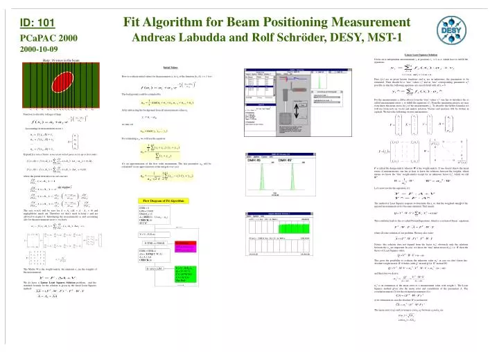
1. Flow Diagram of Fit Algorithm Linear Least Squares Solution Given are n independent measurements yi at positions xi, i=1 to n, which have to fulfill the equations: ITER = 0 LIM = 0.0001 NMAX = 15 A = INIT(U) ; U=(u1,…,un) CHECK(A) SET W’ Harp: 16 wires in the beam Initial Values How to evaluate initial values for the parameters a1 to a4 of the function f(xi;A),i = 1 to n : i = 1 to n, and j = 1 to m < n . Here fj(x) are m given known functions and aj are m unknowns, the parameters to be estimated. Their should be n ‘true’ values yi^ and m ‘true’ corresponding parameters aj^ possible so that the following equations are exactly hold with all vi = 0: The background could be estimated by: . For the measurements yi differ always from the ‘true’ values yi^, one has to introduce the so called measurement errors vi to fulfill the equations (1). From the measuring process we may even know the mean errors s(yi) of the measurements yi. To describe the further formulas we will use from now on vector and matrix notation. Vectors and matrices will be written in capitals. We have the following vectors and matrices: Function to describe voltages of harp: After subtracting the background from all measurement values ui: Accounting for measurement errors v: Y = U - F(X;A) we may set: For estimating a30 we will use the equation: Expand f(x) into a Taylor series at an initial guess set A0 up to first order: If ITER >= NMAX No Solution u1 u2 u3 u4 u5 u6 u7 u8 u9 u10 u11 u12 u13 u14 u15 u16 SET a1=mean(ui) SET a2=a3=a4=0 ITER = ITER+1 DA = LSTQ(Y, W, A) A = A + DA CHECK(A) where the partial derivatives in our case are: It’s an approximation of the first order momentum. The last parameter a40 will be calculated via an approximation of the integral over y(x): F is called the design-matrix whereas W is the weight-matrix. If one doesn’t know the mean errors of measurements, one has at least to know the relations between the weights, which means we know the ‘true’ weight-matrix except for an unknown factor s02, which we call W’: Let’s now rewrite the equations (1): The rest r=r(A) will be zero for A = Ao(DA = A - Ao = 0) and negligiblefor small DA. Therefore we don’t need to keep r and are allowed to neglect it. Introducing the measurements ui and accounting also for the measurement errors vi we have: V = Y – F(X,A) Q = VT·W’·V CA’=(FTW’F)-1 CA = Q·CA’ The End If |DA| < LIM The method of Least Squares requests to determine the aj so, that the weighted sum Q of the squared measurement errors becomes minimal. That means: This condition leads to the so called Normal Equations, which is a system of linear equations: where Ā is the solution of our problem. We may also write: The Matrix W is the weight-matrix, the elements wiare the weights of the measurement. Notice: this solution does not depend from the factor s02, obviously only the relations between the wii are important. In case we know the ‘true’ mean errors s(yi), i.e. W, then the theory of Least Squares states: We do have a LinearLeast SquaresSolution problem, and the standard formula for the solution is given by the linear Least Squares method: This gives the possibility to evaluate the unknown value s02 in case we don’t know the absolute weight-matrix W. It holds (with Q’ instead Q for W’ instead W): and therefore we derive: s02 is an estimation of the mean error of a measurement value with weight 1. The Least Squares method gives also the mean error and correlations of the parameters A. The correlation-matrix CA for the estimated parameters A is: or its estimation in case the absolute W is not known: The mean error s(aj) and covariance cov(aj,ak) between aj andak are: ID: 101Fit Algorithm for Beam Positioning MeasurementPCaPAC 2000 Andreas Labudda and Rolf Schröder, DESY, MST-12000-10-09 (3) (2) .