
Data Warehousing
E N D
Presentation Transcript
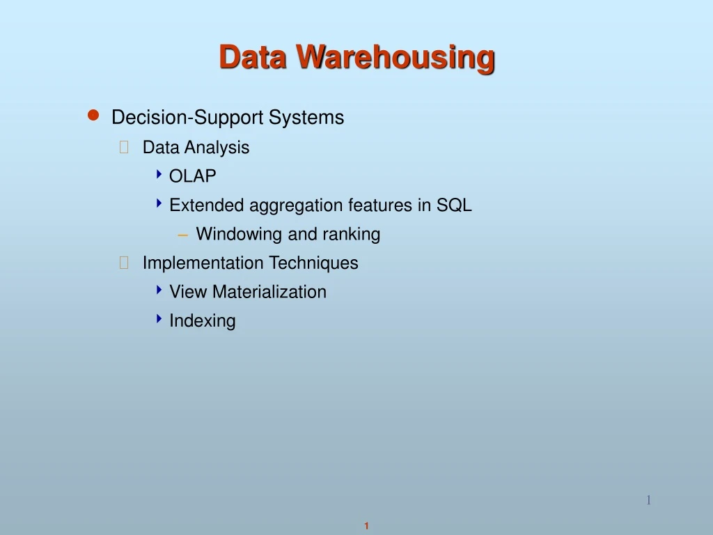
Decision-Support Systems Data Analysis OLAP Extended aggregation features in SQL Windowing and ranking Implementation Techniques View Materialization Indexing Data Warehousing
Decision-support systems are used to make business decisions often based on data collected by on-line transaction-processing systems. Examples of business decisions: what items to stock? What insurance premium to change? Who to send advertisements to? Examples of data used for making decisions Retail sales transaction details Customer profiles (income, age, sex, etc.) Decision Support Systems
Data analysis tasks are simplified by specialized tools and SQL extensions Example tasks For each product category and each region, what were the total sales in the last quarter and how do they compare with the same quarter last year As above, for each product category and each customer category Statistical analysis packages (e.g., : S++) can be interfaced with databases Statistical analysis is a large field will not study it here Data mining seeks to discover knowledge automatically in the form of statistical rules and patterns from Large databases. A data warehouse archives information gathered from multiple sources, and stores it under a unified schema, at a single site. Important for large businesses which generate data from multiple divisions, possibly at multiple sites Data may also be purchased externally Decision-Support Systems: Overview
Composed of four major components: Data Store Component That is, DSS database Data Extraction and Filtering Component Used to extract and validate data taken from operational databases and external data sources End-User Query Tool Used to create queries that access Data Store Component End-User Presentation Tool Component Used to organize and present data Decision-Support Systems: Overview
The Data Warehouse • Integrated, subject-oriented, time-variant, nonvolatile database that provides support for decision making • Growing industry: $8 billion in 1998 • Range from desktop to huge: • Walmart: 900-CPU, 2,700 disk, 23TBTeradata system • Lots of buzzwords, hype • slice & dice, rollup, MOLAP, pivot, ...
more What is a Warehouse? • Collection of diverse data • subject oriented • aimed at executive, decision maker • often a copy of operational data • with value-added data (e.g., summaries, history) • integrated • time-varying • non-volatile
What is a Warehouse? • Collection of tools • gathering data • cleansing, integrating, ... • querying, reporting, analysis • data mining • monitoring, administering warehouse
Client Client Query & Analysis Warehouse Integration Source Source Source Warehouse Architecture Metadata
? Source Source Why a Warehouse? • Two Approaches: • Query-Driven (Lazy) • Warehouse (Eager)
Client Client Mediator Wrapper Wrapper Wrapper Source Source Source Query-Driven Approach
Advantages of Warehousing • High query performance • Queries not visible outside warehouse • Local processing at sources unaffected • Can operate when sources unavailable • Can query data not stored in a DBMS • Extra information at warehouse • Modify, summarize (store aggregates) • Add historical information
Advantages of Query-Driven • No need to copy data • less storage • no need to purchase data • More up-to-date data • Query needs can be unknown • Only query interface needed at sources
Data Marts • Smaller warehouses • Spans part of organization • e.g., marketing (customers, products, sales) • Do not require enterprise-wide consensus • but long term integration problems?
Aggregate functions summarize large volumes of data Online Analytical Processing (OLAP) Interactive analysis of data, allowing data to be summarized and viewed in different ways in an online fashion (with negligible delay) Data that can be modeled as dimension attributes and measure attributes are called multidimensional data. Given a relation used for data analysis, we can identify some of its attributes as measure attributes, since they measure some value, and can be aggregated upon. For instance, the attribute number of the sales relation is a measure attribute, since it measures the number of units sold. Some of the other attributes of the relation are identified as dimension attributes, since they define the dimensions on which measure attributes, and summaries of measure attributes, are viewed. Data Analysis and OLAP
The earliest OLAP systems used multidimensional arrays in memory to store data cubes, and are referred to as multidimensional OLAP (MOLAP) systems. OLAP implementations using only relational database features are called relational OLAP (ROLAP) systems Hybrid systems, which store some summaries in memory and store the base data and other summaries in a relational database, are called hybrid OLAP (HOLAP)systems. OLAP Implementation
Warehouse Schemas • Typically warehouse data is multidimensional, with very large fact tables • Examples of dimensions: item-id, date/time of sale, store where sale was made, customer identifier • Examples of measures: number of items sold, price of items • Dimension values are usually encoded using small integers and mapped to full values via dimension tables • Resultant schema is called a star schema • More complicated schema structures • Snowflake schema: multiple levels of dimension tables • Constellation: multiple fact tables
Terms • Fact table • Dimension tables • Measures
Star Schemas • A star schema is a common organization for data at a warehouse. It consists of: • Fact table : a very large accumulation of facts such as sales. • Often “insert-only.” • Dimension tables : smaller, generally static information about the entities involved in the facts.
Dimension Hierarchies sType store city region è snowflake schema è constellations
The operation of changing the dimensions used in a cross-tab is called pivoting Suppose an analyst wishes to see a cross-tab on item-name and color for a fixed value of size, for example, large, instead of the sum across all sizes. Such an operation is referred to as slicing. The operation is sometimes called dicing, particularly when values for multiple dimensions are fixed. The operation of moving from finer-granularity data to a coarser granularity is called a rollup. The opposite operation - that of moving from coarser-granularity data to finer-granularity data – is called a drill down. Online Analytical Processing
Three-Dimensional Data Cube • A data cube is a multidimensional generalization of a crosstab • Cannot view a three-dimensional object in its entirety • but crosstabs can be used as views on a data cube
Cube Fact table view: Multi-dimensional cube: dimensions = 2
day 2 day 1 3-D Cube Fact table view: Multi-dimensional cube: dimensions = 3
Typical OLAP Queries • Often, OLAP queries begin with a “star join”: the natural join of the fact table with all or most of the dimension tables. • The typical OLAP query will: • Start with a star join. • Select for interesting tuples, based on dimension data. • Group by one or more dimensions. • Aggregate certain attributes of the result.
Aggregates • Add up amounts for day 1 • In SQL: SELECT sum(amt) FROM SALE WHERE date = 1 81
Aggregates • Add up amounts by day • In SQL: SELECT date, sum(amt) FROM SALE GROUP BY date
Another Example • Add up amounts by day, product • In SQL: SELECT date, sum(amt) FROM SALE GROUP BY date, prodId rollup drill-down
Aggregates • Operators: sum, count, max, min, median, ave • “Having” clause • Using dimension hierarchy • average by region (within store) • maximum by month (within date)
rollup drill-down Cube Aggregation Example: computing sums day 2 . . . day 1 129
Cube Operators day 2 . . . day 1 sale(c1,*,*) 129 sale(c2,p2,*) sale(*,*,*)
Extended Cube * day 2 sale(*,p2,*) day 1
day 2 day 1 Aggregation Using Hierarchies customer region country (customer c1 in Region A; customers c2, c3 in Region B)
day 2 day 1 Pivoting Fact table view: Multi-dimensional cube:
OLAP Implementation • Early OLAP systems precomputed all possible aggregates in order to provide online response • Space and time requirements for doing so can be very high • 2n combinations of group by • It suffices to precompute some aggregates, and compute others on demand from one of the precomputed aggregates • Can compute aggregate on (item-name, color) from an aggregate on (item-name, color, size) • For all but a few “non-decomposable” aggregates such as median • is cheaper than computing it from scratch • Several optimizations available for computing multiple aggregates • Can compute aggregate on (item-name, color) from an aggregate on (item-name, color, size) • Can compute aggregates on (item-name, color, size), (item-name, color) and (item-name) using a single sorting of the base data
The table above is an example of a cross-tabulation (cross-tab), also referred to as a pivot-table. A cross-tab is a table where values for one of the dimension attributes form the row headers, values for another dimension attribute form the column headers Other dimension attributes are listed on top Values in individual cells are (aggregates of) the values of the dimension attributes that specify the cell. Cross Tabulation of sales by item-name and color
Relational Representation of Crosstabs • Crosstabs can be represented as relations • The value all is used to represent aggregates • The SQL:1999 standard actually uses null values in place of all • More on this later….