Routing Protocols

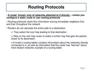
1. Routing Protocols

2. Plan Schedule Report Topic • Aug 16 – Routing (CCNA2) • Aug 23 – LAB • Aug 30- Transport L. • Sep 6– Application L. • Sep 13 – Presentation • Sep 20 – Packet Tracer Exam • Sep 27 – Final • Bluetooth () • xDSL() • RFID () • Ad Hoc Networks () • 3G/4G evolution

3. 5 3 5 2 2 1 3 1 2 1 C D B A E F Viewing Routing as a Policy • Given multiple alternative paths, how to route information to destinations should be viewed as a policy decision • What are some possible policies? • Shortest path (RIP, OSPF) • Load Balanced • Power Aware • QoS routing (satisfies app requirements) • etc

4. Different Approaches • Centralized vs distributed • Centralized simpler, but not practical – central management, congestion, hard to scale… • Source-based vs hop by hop • Source puts path in header, can be more robust, but difficult to scale • Single vs multiple path • Router keeps multiple paths for each destination • State-dependent vs state-independent • Compute routes based on current network load (e.g. delay) • Periodic versus On-demand • On-demand proposed for wireless networks

5. Internet Routing • Internet topology roughly organized as a two level hierarchy • First lower level – autonomous systems (AS’s) • AS: region of network under a single administrative domain • Each AS runs an intra-domain routing protocol • Distance Vector, e.g., Routing Information Protocol (RIP) • Link State, e.g., Open Shortest Path First (OSPF) • Possibly others • Second level – inter-connected AS’s • Between AS’s runs inter-domain routing protocols, e.g., Border Gateway Routing (BGP) • Standard today, BGP-4

6. Example Interior router BGP router AS-1 AS-3 AS-2

7. Why do we Need the Concept of AS or Domain? • Routing algorithms are not efficient enough to deal with the size of the entire Internet • Different organizations may want different internal routing policies • Allow organizations to hide their internal network configurations from outside • Allow organizations to choose how to route across multiple organizations (BGP) • Basically, easier to compute routes, more flexibility, more autonomy/independence

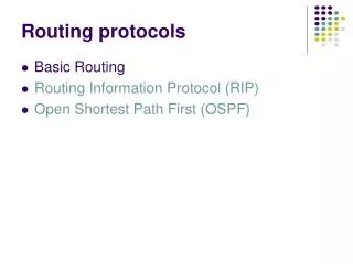
8. Outline • Two intra-domain routing protocols • Both try to achieve the “shortest path” routing policy • Quite commonly used • OSPF: Based on Link-State routing algorithm • RIP: Based on Distance-Vector routing algorithm

9. Intra-domain Routing Protocols • Based on unreliable datagram delivery • Distance vector • Routing Information Protocol (RIP), based on Bellman-Ford algorithm • Each neighbor periodically exchange reachability information to its neighbors • Minimal communication overhead, but it takes long to converge, i.e., in proportion to the maximum path length • Link state • Open Shortest Path First (OSPF), based on Dijkstra’s algorithm • Each router periodically floods immediate reachability information to other routers • Fast convergence, but high communication and computation overhead

10. 5 3 5 2 2 1 3 1 2 1 C D B A E F Routing on a Graph • Goal: determine a “good” path through the network from source to destination • Good often means the shortest path • Network modeled as a graph • Routers  nodes • Link edges • Edge cost: delay, congestion level,…

11. 5 3 5 2 2 1 3 1 2 1 C D A E B F Link State Routing (OSPF): Flooding • Each node knows its connectivity and cost to a direct neighbor • Every node tells every other node this local connectivity/cost information • Via flooding • In the end, every node learns the complete topology of the network • E.g. A floods message A connected to B cost 2 A connected to D cost 1 A connected to C cost 5

12. Link State Flooding Example 5 5 5 5 7 7 7 7 4 4 4 4 8 8 8 8 6 6 6 6 11 11 11 11 2 2 2 2 10 10 10 10 3 3 3 3 1 1 1 1 13 13 13 13 12 12 12 12

13. Dijkstra’s algorithm Net topology, link costs known to all nodes Accomplished via “link state flooding” All nodes have same info Compute least cost paths from one node (‘source”) to all other nodes Repeat for all sources Notations c(i,j): link cost from node i to j; cost infinite if not direct neighbors D(v): current value of cost of path from source to node v p(v): path from source to v S: set of nodes whose least cost path definitively known A Link State Routing Algorithm

14. Dijsktra’s Algorithm (A “Greedy” Algorithm) 1 Initialization: 2 S = {A}; 3 for all nodes v 4 if v adjacent to A 5 then D(v) = c(A,v); 6 else D(v) = ; 7 8 Loop 9 find w not in S such that D(w) is a minimum; 10 add w to S; 11 update D(v) for all v adjacent to w and not in S: 12 D(v) = min( D(v), D(w) + c(w,v) ); // new cost to v is either old cost to v or known // shortest path cost to w plus cost from w to v 13 until all nodes in S;

15. C D E A B F Example: Dijkstra’s Algorithm D(B),p(B) 2,AB D(D),p(D) 1,AD D(C),p(C) 5,AC D(E),p(E) Step 0 1 2 3 4 5 start S A D(F),p(F) 1 Initialization: 2 S = {A}; 3 for all nodes v 4 if v adjacent to A 5 then D(v) = c(A,v); 6 else D(v) = ; … 5 3 5 2 2 1 3 1 2 1

16. C D E A B F Example: Dijkstra’s Algorithm D(B),p(B) 2,AB D(D),p(D) 1,AD D(C),p(C) 5,AC 4,ADC D(E),p(E) 2,ADE Step 0 1 2 3 4 5 start S A AD D(F),p(F) • … • 8 Loop • 9 find w not in S s.t. D(w) is a minimum; • 10 add w to S; • update D(v) for all v adjacent • to w and not in S: • 12 D(v) = min( D(v), D(w) + c(w,v) ); • 13 until all nodes in S; 5 3 5 2 2 1 3 1 2 1

17. C D E A B F Example: Dijkstra’s Algorithm D(B),p(B) 2,AB D(D),p(D) 1,AD D(C),p(C) 5,AC 4,ADC 3,ADEC D(E),p(E) 2,ADE Step 0 1 2 3 4 5 start S A AD ADE D(F),p(F) 4,ADEF • … • 8 Loop • 9 find w not in S s.t. D(w) is a minimum; • 10 add w to S; • update D(v) for all v adjacent • to w and not in S: • 12 D(v) = min( D(v), D(w) + c(w,v) ); • 13 until all nodes in S; 5 3 5 2 2 1 3 1 2 1

18. C D E A B F Example: Dijkstra’s Algorithm D(B),p(B) 2,AB D(D),p(D) 1,AD D(C),p(C) 5,AC 4,ADC 3,ADEC D(E),p(E) 2,ADE Step 0 1 2 3 4 5 start S A AD ADE ADEB D(F),p(F) 4,ADEF 5 • … • 8 Loop • 9 find w not in S s.t. D(w) is a minimum; • 10 add w to S; • update D(v) for all v adjacent • to w and not in S: • 12 D(v) = min( D(v), D(w) + c(w,v) ); • 13 until all nodes in S; 3 5 2 2 1 3 1 2 1

19. C D E A B F Example: Dijkstra’s Algorithm D(B),p(B) 2,AB D(D),p(D) 1,AD D(C),p(C) 5,AC 4,ADC 3,ADEC D(E),p(E) 2,ADE Step 0 1 2 3 4 5 start S A AD ADE ADEB ADEBC D(F),p(F) 4,ADEF 5 • … • 8 Loop • 9 find w not in S s.t. D(w) is a minimum; • 10 add w to S; • update D(v) for all v adjacent • to w and not in S: • 12 D(v) = min( D(v), D(w) + c(w,v) ); • 13 until all nodes in S; 3 5 2 2 1 3 1 2 1

20. C D E A B F Example: Dijkstra’s Algorithm D(B),p(B) 2,AB D(D),p(D) 1,AD D(C),p(C) 5,AC 4,ADC 3,ADEC D(E),p(E) 2,ADE Step 0 1 2 3 4 5 start S A AD ADE ADEB ADEBC ADEBCF D(F),p(F) 4,ADEF 5 • … • 8 Loop • 9 find w not in S s.t. D(w) is a minimum; • 10 add w to S; • update D(v) for all v adjacent • to w and not in S: • 12 D(v) = min( D(v), D(w) + c(w,v) ); • 13 until all nodes in S; 3 5 2 2 1 3 1 2 1

21. Distance Vector Routing (RIP) • What is a distance vector? • Current best known cost to get to a destination • Idea: Exchange distance vectors among neighbors to learn about lowest cost paths Node C Note no vector entry for C itself At the beginning, distance vector only has information about directly attached neighbors, all other dests have cost  Eventually the vector is filled

22. wait for (change in local link cost or msg from neighbor) recompute distance table if least cost path to any dest has changed, notify neighbors Distance Vector Routing Each node: • Each local iteration caused by: • Local link cost change • Message from neighbor: its least cost path change from neighbor to destination • Each node notifies neighbors only when its least cost path to any destination changes • Neighbors then notify their neighbors if necessary

23. Distance Vector Algorithm (cont’d) • 1 Initialization: • 2 for all nodes V do • 3 ifV adjacent to A • 4 D(A, V, V) = c(A,V); /* Distance from A to V via neighbor V */ • 5 else • D(A, V, *) = ∞; • loop: • 8 wait (until A sees a link cost change to neighbor V • 9 or until A receives update from neighbor V) • 10 if (c(A,V) changes by d) • 11 for all destinations Y through Vdo • 12 D(A,Y, V) = D(A,Y,V) + d • 13 else if (update D(V, Y) received from V) • /* shortest path from V to some Y has changed */ • 14 D(A,Y,V) = c(A,V) + D(V, Y); • 15 if (there is a new minimum for destination Y) • 16 send D(A, Y) to all neighbors /* D(A,Y) denotes the min D(A,Y,*) */ • 17 forever

24. C D B A Example: Distance Vector Algorithm Node A Node B 3 2 1 1 7 Node C Node D • 1 Initialization: • 2 for all nodes V do • 3 ifV adjacent to A • 4 D(A, V, V) = c(A,V); • else • D(A, V, *) = ∞; • …

25. D C B A Example: 1st Iteration (C  A) Node A Node B 3 2 1 1 7 • loop: • … • 13 else if (update D(V, Y) received from V) • 14 D(A,Y,V) = c(A,V) + D(V, Y); • 15 if (there is a new min. for destination Y) • 16 send D(A, Y) to all neighbors • 17 forever D(A,D,C) = c(A, C) + D(C,D) = 7 + 1 = 8 (D(C,A), D(C,B), D(C,D)) Node C Node D

26. D C B A Example: 1st Iteration (BA, CA) Node A Node B 3 2 1 1 7 D(A,D,B) = c(A,B) + D(B,D) = 2 + 3 = 5 D(A,C,B) = c(A,B) + D(B,C) = 2 + 1 = 3 Node C Node D • loop: • … • 13 else if (update D(V, Y) received from V) • 14 D(A,Y,V) = c(A,V) + D(V, Y) • 15 if (there is a new min. for destination Y) • 16 send D(A, Y) to all neighbors • 17 forever

27. C D B A Example: End of 1st Iteration Node A Node B 3 2 1 1 7 • loop: • … • 13 else if (update D(V, Y) received from V) • 14 D(A,Y,V) = c(A,V) + D(V, Y); • 15 if (there is a new min. for destination Y) • 16 send D(A, Y) to all neighbors • 17 forever Node C Node D

28. C D B A Example: End of 2nd Iteration Node A Node B 3 2 1 1 7 • loop: • … • 13 else if (update D(V, Y) received from V) • 14 D(A,Y,V) = c(A,V) + D(V, Y); • 15 if (there is a new min. for destination Y) • 16 send D(A, Y) to all neighbors • 17 forever Node C Node D

29. C D B A Nothing changes  algorithm terminates Example: End of 3rdIteration Node A Node B 3 2 1 1 7 • loop: • … • 13 else if (update D(V, Y) received from V) • 14 D(A,Y,V) = c(A,V) + D(V, Y); • 15 if (there is a new min. for destination Y) • 16 send D(A, Y) to all neighbors • 17 forever Node C Node D

30. 1 4 1 50 C A B Distance Vector: Link Cost Changes 7 loop: 8 wait (until A sees a link cost change to neighbor V 9 or until A receives update from neighbor V) 10 if (c(A,V) changes by d) 11 for all destinations Y through Vdo 12 D(A,Y,V) = D(A,Y,V) + d 13 else if (update D(V, Y) received from V) 14 D(A,Y,V) = c(A,V) + D(V, Y); 15 if (there is a new minimum for destination Y) 16 send D(A, Y) to all neighbors 17 forever “good news travels fast” Node B Node C time Link cost changes here Algorithm terminates

31. 60 4 1 50 C A B Distance Vector: Count to Infinity Problem 7 loop: 8 wait (until A sees a link cost change to neighbor V 9 or until A receives update from neighbor V) 10 if (c(A,V) changes by d) 11 for all destinations Y through Vdo 12 D(A,Y,V) = D(A,Y,V) + d ; 13 else if (update D(V, Y) received from V) 14 D(A,Y,V) = c(A,V) + D(V, Y); 15 if (there is a new minimum for destination Y) 16 send D(A, Y) to all neighbors 17 forever “bad news travels slowly” Node B Node C … time Link cost changes here; recall that B also maintains shortest distance to A through C, which is 6. Thus D(B, A) becomes 6 !

32. Per node message complexity LS: O(n*d) messages; n – number of nodes; d – degree of node DV: O(d) messages; where d is node’s degree Complexity LS: O(n2) with O(n*d) messages (with naïve priority queue) DV: convergence time varies may be routing loops count-to-infinity problem Robustness: what happens if router malfunctions? LS: node can advertise incorrect link cost each node computes only its own table DV: node can advertise incorrect path cost each node’s table used by others; error propagate through network Link State vs. Distance Vector

33. Practice Problem 1. Run Dijkstra fromNode B 2. Run Bellman-Ford fromNode B

34. Dijkstra from Node B

35. Distance Vector at Node B

36. Homework: To be hand in next week 1. Explain the following methods used to solve the Count-to-Infinity problem Split Horizon - Poison Reverse 2. Run Dijkstra from Node D and H 3. Run Bellman-Ford from Node D and H

37. Dijkstra from Node D

38. Distance Vector at Node D

39. Dijkstra from Node H

40. Distance Vector at Node H