Download

1 / 14
160 likes | 274 Views
This guide provides an overview of binomial distributions, highlighting the four key commandments: (1) a fixed number of trials, (2) each trial has two possible outcomes, (3) the probability of success is constant, and (4) trials are independent. It details key formulas for calculating probabilities, including the probability distribution function (PDF) and cumulative distribution function (CDF). Real-world examples in sports statistics illustrate the application of binomial probability, along with guidance on using normal approximation when sample sizes are large.

E N D
Binomial Distributions Section 8.1
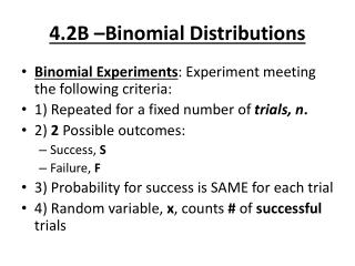
The 4 “Commandments” of Binomial Distributions • There are n trials. • Each trial results in a success or a failure. • The probability of a success, p, is constant from trial to trial. • The trials are independent. -Knowing the result of one observation tells you nothing about the other observations.
Sampling Distribution of a Count • Choose an SRS of size n from a population with proportion p of successes. When the population is much larger than the sample, the count X of successes in the sample has approximately the binomial distribution with parameters n and p. • Essentially, it is sometimes sufficient for outcomes of an event to be “close enough” to independent to use binomial calculations.
Key formulas If data fits binomial setting, then random variable X = number of successes is called a binomial random variable. And the probability distribution of X is called a binomial distribution. We represent this distribution as B(n,p).
P.D.F. • Given a discrete random variable X, the probability distribution function assigns a probability to each value of X. The probabilities must satisfy the rules for probabilities given in Chapter 6…
Rules of Probability--Chapter 6 • Rule 1: 0 ≤ P(A) ≤ 1 for any event A. • Rule 2: P(S) = 1. • Rule 3: complement rule; for any event A, • P(AC) = 1 – P(A) • Rule 4: Addition rule: • P(A or B) = P(A) + P(B) – P(A and B) • Rule 5: Multiplication rule: • P(A and B) = P(A)P(B|A)
C.D.F. • Given a random variable X, the cumulative distribution function of X calculates the sum of the probabilities for 0, 1, 2, …, up to the value X. That is, it calculates the probability of obtaining at most X successes in n trials.
Calculator Tips • To determine P(X = x) Use binompdf(n, p, x): where n is the number of observations, p is the probability of success. • To determine P(X ≤ x) Use binomcdf(n, p, x): where n is the number of observations, p is the probability of success. • To determine P(X > x) Use 1-binomcdf(n, p, x): where n is the number of observations, p is the probability of success. • To determine P(X < x) Use binomcdf(n, p, x-1): where n is the number of observations, p is the probability of success.
Binomial Setting Example A baseball pitcher throws 30 pitches in an inning. The pitcher throws a strike 60% of the time. • Is this binomial setting? Let’s check! 1. Can each observation be categorized as a success or failure? YES: Throwing a strike is a success, throwing a ball (not a strike) is a failure. 2. Are there a fixed number of observations? YES: The pitcher throws 30 pitches. 3. Are all n of the observations independent? YES: While it is possible that one pitch impacts another, it is still safe to assume that they are independent. 4. Is the probability of success the same for each observation? YES: While a pitcher may get tired as the game wears on, thus changing the probability of throwing a strike, it is safe to assume that throughout a season, the probability of throwing a strike is the same.
Binomial Setting Example (cont.) np = (30)(0.6) = 18 B) How many strikes does the pitcher expect to throw? C) What is the standard deviation? D) What is the probability that the pitcher throws exactly 21 strikes in the inning? E) What is the probability that he throws 15 or fewer strikes? F) What is the probability that he throws more than 11 strikes? binompdf(30, 0.6, 21) ≈ 0.0823 binomcdf(30, 0.6, 15) ≈ 0.1754 1 – binomcdf(30, 0.6, 11) ≈ 0.9917
What if we are between values? • Consider the pitcher scenario. • What is the probability that he throws between 12 and 20 strikes? • We can’t do binomcdf directly or 1-binomcdf • Try: • binomcdf(30, 0.6, 20) – binomcdf(30, 0.6, 11) • =0.8154
Normal Approximation tothe Binomial Distribution • If X is a count having the binomial distribution with parameters n and p, then when n is larger, X is approximately N(np, ). • As a rule of thumb, we can use this approximation when np ≥ 10 and n(1-p) ≥ 10. • Essentially, we can use this approximation if we expect at least 10 successes and 10 failures. • The accuracy of the Normal Approximation improves as the sample size increases • It is most accurate for any fixed n when p is close to ½ and least accurate when p is near 0 or 1 and the distribution is skewed.
Normal Approximation Example • Many local polls of public opinion use samples of size 400 to 800. Consider a poll of 400 adults in Atlanta that asks the question “Do you approve of President Bush’s response to the World Trade Center terrorists attacks in September 2001?” Suppose we know that President Bush’s approval rating on this issue nationally is 92% a week after the incident. • What is the random variable X? • X = the number of polled people that approve of Bush’s response
Normal Approx. Ex. Continued • Is X binomial? • n = 400, approve = success & not = failure, if polled separately should be independent, with random polling probability should be same for each person polled • Calculate the binomial probability that at most 358 of the 400 adults in the Atlanta poll answer “Yes” to this question. • binomcdf(400, 0.92, 358) ≈ 0.0441 • Find the expected number of people in the sample who indicate approval. Find the standard deviation of X. • We expect with • Perform a normal approximation to the question above if possible. • np=368≥10, n(1-p)=32≥10, normalcdf(0, 358, 368, ) ≈ 0.0327