Download
1 / 63
640 likes | 1.11k Views
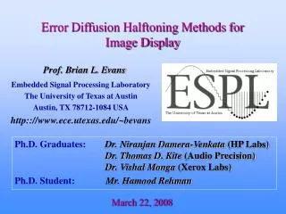
Error Diffusion Halftoning Methods for High-Quality Printed and Displayed Images. Prof. Brian L. Evans. Embedded Signal Processing Laboratory The University of Texas at Austin Austin, TX 78712-1084 USA http:://www.ece.utexas.edu/~bevans.

E N D
Error Diffusion Halftoning Methods forHigh-Quality Printed and Displayed Images Prof. Brian L. Evans Embedded Signal Processing Laboratory The University of Texas at Austin Austin, TX 78712-1084 USA http:://www.ece.utexas.edu/~bevans Ph.D. Graduates: Dr. Niranjan Damera-Venkata (HP Labs) Dr. Thomas D. Kite (Audio Precision) Graduate Student: Mr. Vishal Monga Other Collaborators: Prof. Alan C. Bovik (UT Austin) Prof. Wilson S. Geisler (UT Austin) Last modified November 7, 2002
Outline • Introduction • Grayscale halftoning methods • Modeling grayscale error diffusion • Compensation for sharpness • Visual quality measures • Compression of error diffused halftones • Color error diffusion halftoning for display • Optimal design • Linear human visual system model • Conclusion
Introduction Need for Digital Image Halftoning • Examples of reduced grayscale/color resolution • Laser and inkjet printers ($9.3B revenue in 2001 in US) • Facsimile machines • Low-cost liquid crystal displays • Halftoning is wordlength reduction for images • Grayscale: 8-bit to 1-bit (binary) • Color displays: 24-bit RGB to 12-bit RGB (e.g. PDA/cell) • Color displays: 24-bit RGB to 8-bit RGB (e.g. cell phones) • Color printers: 24-bit RGB to CMY (each color binarized) • Halftoning tries to reproduce full range of gray/ color while preserving quality & spatial resolution
Introduction Original Image Threshold at Mid-Gray Dispersed Dot Screening Clustered DotScreening Stucki Error Diffusion Floyd SteinbergError Diffusion Conversion to One Bit Per Pixel: Spatial Domain
Introduction Dispersed Dot Screening Threshold at Mid-Gray Original Image Clustered DotScreening Stucki Error Diffusion Floyd SteinbergError Diffusion Conversion to One Bit Per Pixel: Magnitude Spectra
Introduction Need for Speed for Digital Halftoning • Third-generation ultra high-speed printer (CMYK) • 100 pages per minute, 600 lines per inch, 4800 dots/inch/line • Output data rate of 7344 MB/s (HDTV video is ~96 MB/s) • Desktop color printer (CMYK) • 24 pages per minute, 600 lines/inch, 600 dots/inch/line • Output data rate of 220 MB/s (NTSC video is ~24 MB/s) • Parallelism • Screening: pixel-parallel, fast, and easy to implement(2 byte reads, 1 compare, and 1 bit write per binary pixel) • Error diffusion: row-parallel, better results on some media(5 byte reads, 1 compare, 4 MACs, 1 byte and 1 bit write per binary pixel)
Outline • Introduction • Grayscale halftoning methods • Modeling grayscale error diffusion • Compensation for sharpness • Visual quality measures • Compression of error diffused halftones • Color error diffusion halftoning for display • Optimal design • Linear human visual system model • Conclusion
Grayscale Halftoning Screening (Masking) Methods • Periodic array of thresholds smaller than image • Spatial resampling leads to aliasing (gridding effect) • Clustered dot screening is more resistant to ink spread • Dispersed dot screening has higher spatial resolution • Blue noise masking uses large array of thresholds Clustered dot mask Dispersed dot mask
Grayscale Halftoning difference threshold u(m) Error Diffusion x(m) b(m) _ 7/16 + 3/16 5/16 1/16 _ + e(m) shape error compute error Spectrum Grayscale Error Diffusion • Shape quantization noise into high frequencies • Design of error filter key to quality • Not a screening technique current pixel 2-D sigma-delta modulation [Anastassiou, 1989] weights
Grayscale Halftoning Simple Noise Shaping Example • Two-bit output device and four-bit input words • Going from 4 bits down to 2 increases noise by ~ 12 dB • Shaping eliminates noise at DC at expense of increased noise at high frequency. 4 2 Average output = ¼ (10+10+10+11)=1001 Input words To output device 4-bit resolution at DC! 2 2 Added noise 1 sample delay Assume input = 1001 constant 12 dB (2 bits) Time Input Feedback Sum Output 1 1001 00 1001 10 2 1001 01 1010 10 3 1001 10 1011 10 4 1001 11 1100 11 f Periodic If signal is in this band, then you are better off
Grayscale Halftoning Direct Binary Search (Iterative) • Practical upper bound on halftone quality • Minimize mean-squared error between lowpass filtered versions of grayscale and halftone images • Lowpass filter is based on a linear shift-invariant model of human visual system (a.k.a. contrast sensitivity function) • Each iteration visits every pixel [Analoui & Allebach, 1992] • At each pixel, consider toggling pixel or swapping it with each of its 8 nearest neighbors that differ in state from it • Terminate when if no pixels are changed in an iteration • Relatively insensitive to initial halftone provided that it is not error diffused [Lieberman & Allebach, 2000]
Contrast at particular spatial frequency for visibility Bandpass: non-dim backgrounds [Manos & Sakrison, 1974; 1978] Lowpass: high-luminance office settings with low-contrast images [Georgeson & G. Sullivan, 1975] Modified lowpass version[e.g. J. Sullivan, Ray & Miller, 1990] Angular dependence: cosine function [Sullivan, Miller & Pios, 1993] Exponential decay [Näsäsen, 1984] Näsänen’s is best for direct binary search[Kim & Allebach, 2002] Grayscale Halftoning Many Possible Contrast Sensitivity Functions
Grayscale Halftoning Digital Halftoning Methods Clustered Dot Screening AM Halftoning Dispersed Dot Screening FM Halftoning Error Diffusion FM Halftoning 1976 Blue-noise MaskFM Halftoning 1993 Green-noise Halftoning AM-FM Halftoning 1992 Direct Binary Search FM Halftoning 1992
Outline • Introduction • Grayscale halftoning methods • Modeling grayscale error diffusion • Compensation for sharpness • Visual quality measures • Compression of error diffused halftones • Color error diffusion halftoning for display • Optimal design • Linear human visual system model • Conclusion
Modeling Grayscale Error Diffusion current pixel Floyd-Steinbergweights 7/16 3/16 5/16 1/16 Floyd-Steinberg Grayscale Error Diffusion Original Halftone u(m) x(m) b(m) _ + _ + shape error e(m)
Modeling Grayscale Error Diffusion Q(x) 255 x 0 0 128 255 Ks u(m) b(m) Q(•) Modeling Grayscale Error Diffusion • Goal: Model sharpening and noise shaping • Sigma-delta modulation analysis Linear gain model for quantizer in 1-D[Ardalan and Paulos, 1988] Apply linear gain model in 2-D[Kite, Evans & Bovik, 1997] • Uses of linear gain model Compensation of frequency distortion Visual quality measures Ks us(m) us(m) Signal Path n(m) un(m) un(m) + n(m) Noise Path
Image Floyd Stucki Jarvis Modeling Grayscale Error Diffusion barbara 2.01 3.62 3.76 boats 1.98 4.28 4.93 lena 2.09 4.49 5.32 mandrill 2.03 3.38 3.45 Average 2.03 3.94 4.37 Linear Gain Model for Quantizer • Best linear fit for Ks between quantizer input u(i,j) and halftone b(i,j) • Does not vary much for Floyd-Steinberg • Can use average value to estimate Ks from only error filter • Sharpening: proportional to Ks Value of Ks: Floyd Steinberg < Stucki < Jarvis
Modeling Grayscale Error Diffusion STF NTF 2 1 1 w w w -w1 -w1 -w1 w1 w1 w1 Also, let Ks = 2 (Floyd-Steinberg) Pass low frequencies Enhance high frequencies Highpass response(independent of Ks ) Linear Gain Model for Error Diffusion n(m) Quantizermodel x(m) u(m) b(m) Ks _ + f(m) _ • Lowpass H(z) explainsnoise shaping + e(m)
Modeling Grayscale Error Diffusion L b(m) u(m) x(m) _ + _ + e(m) Compensation of Sharpening • Adjust by threshold modulation [Eschbach & Knox, 1991] • Scale image by gain L and add it to quantizer input • For L (-1,0], higher value of L, lower the compensation • No compensation when L = 0 • Low complexity: one multiplication, one addition per pixel
Modeling Grayscale Error Diffusion Compensation of Sharpening • Flatten signal transfer function [Kite, Evans, Bovik, 2000] Globally optimum value of L to compensate for sharpening of signal components in halftone based on linear gain model Ksis chosen as linear minimum mean squared error estimator of quantizer output Assumes that input and output of quantizer are jointly wide sense stationary stochastic processes Use linear minimum mean squared error estimator for quantizer to adapt L to allow other types of quantizers[Damera-Venkata and Evans, 2001]
Modeling Grayscale Error Diffusion Visual Quality Measures [Kite, Evans, Bovik, 2000] • Impact of noise on human visual system Signal-to-noise (SNR) measures appropriate when noise is additive and signal independent Create unsharpened halftone y[m1,m2] with flat signal transfer function using threshold modulation Weight signal/noise by contrast sensitivity function C[k1,k2] Floyd-Steinberg > Stucki > Jarvis at all viewing distances
Outline • Introduction • Grayscale halftoning methods • Modeling grayscale error diffusion • Compensation for sharpness • Visual quality measures • Compression of error diffused halftones • Color error diffusion halftoning for display • Optimal design • Linear human visual system model • Conclusion
JBIG2 standard (Dec. 1999) Binary document printing, faxing, scanning, storage Lossy and lossless coding Models for text, halftone, and generic regions Lossy halftone compression Preserve local average gray level not halftone Periodic descreening High compression of ordered dither halftones Compression of Error Diffused Halftones Generate (M2+1) patterns ofsize M x M from a clustereddot threshold mask Construct Pattern Dictionary Lossless Encoder JBIG2 bitstream Halftone Compute Indices into Dictionary Count black dots in each M x M block of input Range of indices: 0... M2+1 Joint Bi-Level Experts Group
JBIG2 Halftone Compression Model • JBIG2 assumes that halftones were produced by a small periodic screen • Stochastic halftones are aperiodic Existing JBIG-26.1 : 1 Proposed Method 6.6 : 1
Compression of Error Diffused Halftones Lossy Compression of Error Diffused Halftones • Proposed method [Valliappan, Evans, Tompkins, Kossentini, 1999] • Reduce noise and artifacts • Achieve higher compression ratios • Low implementation complexity High Quality Ratio 6.6 : 1 WSNR 18.7 dB LDM 0.116 High Compression Ratio 9.9 : 1 WSNR 14.0 dB LDM 0.158 512 x 512 Floyd-Steinberg halftoneof barbara image
Compression of Error Diffused Halftones Lossy Compression of Error Diffused Halftones • Fast conversion of error diffused halftones to screened halftones with rate-distortion tradeoffs [Valliappan, Evans, Tompkins, Kossentini, 1999] • 3 x 3 lowpass • zeros at Nyquist • reduces noise • 2n coefficients • modified multilevel Floyd Steinberg • error diffusion • L sharpening factor Prefilter Decimator Quantizer Lossless Encoder JBIG2 bitstream Halftone graylevels 2 17 16 M2 + 1 N • M x M lowpass averaging filter • downsample by M x M Symbol Dictionary Free Parameters L sharpening M downsamping factor N grayscale resolution • N patterns • size M x M • may be angled • clustered dot
Compression of Error Diffused Halftones Rate-Distortion Tradeoffs Linear Distortion Measure for downsampling factorM { 2, 3, 4, 5, 6, 7, 8} Weighted SNR for downsampling factorM { 2, 3, 4, 5, 6, 7, 8}(linear distortion removed)
Outline • Introduction • Grayscale halftoning methods • Modeling grayscale error diffusion • Compensation for sharpness • Visual quality measures • Compression of error diffused halftones • Color error diffusion halftoning for display • Optimal design • Linear human visual system model • Conclusion
Color Error Diffusion YUV to RGB Conversion Color Monitor Display Example (Palettization) • YUV color space • Luminance (Y) and chrominance (U,V) channels • Widely used in video compression standards • Human visual system has lowpass response to Y, U, and V • Display YUV on lower-resolution RGB monitor: use error diffusion on Y, U, V channels separably u(m) b(m) 24-bit YUV video 12-bit RGB monitor x(m) + _ _ + RGB to YUV Conversion h(m) e(m)
Color Error Diffusion Non-Separable Color Halftoning for Display • Input image has a vector of values at each pixel (e.g. vector of red, green, and blue components) Error filter has matrix-valued coefficients Algorithm for adaptingmatrix coefficientsbased on mean-squarederror in RGB space[Akarun, Yardimci, Cetin, 1997] • Design problem Given a human visual system model, find the color error filter that minimizes average visible noise power subject to diffusion constraints u(m) x(m) b(m) _ + _ t(m) e(m) +
Color Error Diffusion linear model of human visual system matrix-valued convolution Optimal Design of the Matrix-Valued Error Filter • Develop matrix gain model with noise injection n(m) • Optimize error filter for shaping Subject to diffusion constraints where
Color Error Diffusion Matrix Gain Model for the Quantizer • Replace scalar gain w/ matrix [Damera-Venkata & Evans, 2001] • Noise uncorrelated with signal component of quantizer input • Convolution becomes matrix–vector multiplication in frequency domain u(m) quantizer inputb(m) quantizer output In one dimension Noisecomponentof output Signalcomponentof output
Color Error Diffusion Linear Color Vision Model • Pattern-color separable model [Poirson and Wandell, 1993] • Forms the basis for Spatial CIELab [Zhang and Wandell, 1996] • Pixel-based color transformation B-W R-G B-Y Opponent representation Spatial filtering
Color Error Diffusion Linear Color Vision Model • Undo gamma correction on RGB image • Color separation • Measure power spectral distribution of RGB phosphor excitations • Measure absorption rates of long, medium, short (LMS) cones • Device dependent transformation C from RGB to LMS space • Transform LMS to opponent representation using O • Color separation may be expressed as T = OC • Spatial filtering included using matrix filter • Linear color vision model is a diagonal matrix where
Color Error Diffusion Sample images and optimum coefficients for sRGB monitor available at: http://signal.ece.utexas.edu/~damera/col-vec.html Original Image
Color Error Diffusion Floyd-Steinberg Optimum Filter
Color Error Diffusion C1 C2 C3 Representation inarbitrary color space Spatial filtering Generalized Linear Color Vision Model • Separate image into channels/visual pathways • Pixel based linear transformation of RGB into color space • Spatial filtering based on HVS characteristics & color space • Best color space/HVS model for vector error diffusion? [Monga, Geisler and Evans, 2003]
Color Error Diffusion Eye more sensitive to luminance; reduce chrominance bandwidth Color Spaces • Desired characteristics • Independent of display device • Score well in perceptual uniformity [Poynton color FAQ http://comuphase.cmetric.com] • Approximately pattern color separable [Wandell et al., 1993] • Candidate linear color spaces • Opponent color space [Poirson and Wandell, 1993] • YIQ: NTSC video • YUV: PAL video • Linearized CIELab [Flohr, Bouman, Kolpatzik, Balasubramanian, Carrara, Allebach, 1993]
Color Error Diffusion Monitor Calibration • How to calibrate monitor? sRGB standard default RGB space by HP and Microsoft Transformation based on an sRGB monitor (which is linear) • Include sRGB monitor transformation T: sRGB CIEXYZ Opponent Representation[Wandell & Zhang, 1996] Transformations sRGB YUV, YIQ from S-CIELab Code at http://white.stanford.edu/~brian/scielab/scielab1-1-1/ • Including sRGB monitor into model enables Web-based subjective testing http://www.ece.utexas.edu/~vishal/cgi-bin/test.html
Color Error Diffusion Spatial Filtering • Opponent [Wandell, Zhang 1997] Data in each plane filtered by 2-D separable spatial kernels • Linearized CIELab, YUV, and YIQ Luminance frequency response [Näsänen and Sullivan, 1984] L average luminance of display r radial spatial frequency Chrominance frequency response [Kolpatzik and Bouman, 1992] Chrominance response allows more low frequency chromatic error not to be perceived vs. luminance response
Color Error Diffusion Subjective Testing • Based on paired comparison task • Observer chooses halftone that looks closer to original • Online at www.ece.utexas.edu/~vishal/cgi-bin/test.html • In decreasing subjective quality Linearized CIELab > > Opponent > YUV YIQ halftone A original halftone B
Conclusion Color Error Diffusion • Design of “optimal” color noise shaping filters • We use the matrix gain model [Damera-Venkata and Evans, 2001] • Predicts sharpening • Predicts shaped color halftone noise • Solve for best error filter that minimizes visually weighted average color halftone noise energy • Improve numerical stability of descent procedure • Choice of linear color space • Linear CIELab gives best objective and subjective quality • Future work in finding better transformations • Use color management to generalize device characterization and viewing conditions
Grayscale andcolor methods Screening Classical diffusion Edge enhanced diff. Green noise diffusion Block diffusion Figures of merit Peak SNR Weighted SNR Linear distortion measure Universal quality index Conclusion Image Halftoning Toolbox 1.1 Figures of Merit http://www.ece.utexas.edu/~bevans/projects/halftoning/toolbox
Grayscale Halftoning Problems with Error Diffusion • Objectionable artifacts • Scan order affects results • “Worminess” visible in constant graylevel areas • Image sharpening • Larger error filters due to [Jarvis, Judice & Ninke, 1976] and[Stucki, 1980] reduce worminess and sharpen edges • Sharpening not always desirable: may be adjustable by prefiltering based on linear gain model [Kite, Evans, Bovik, 2000] • Computational complexity • Larger error filters require more operations per pixel • Push towards simple schemes for fast printing
Grayscale Halftoning Correcting Artificial Textures [Marcu, 1999] • False textures in shadow and highlight regions • Place dot if minimum distance constraint is met • Raster scan • Avoids computing geometric distance • Scans halftoned pixels in radius of the current pixel • Radius proportional to distance of pixel value from midgray • Scanned pixel location offsets obtained by lookup tables • One lookup table gives number of pixels to scan (256 entries) • One lookup table gives offsets (256 entries) • Affects grayscale values [1, 39] and [216, 254]
Grayscale Halftoning Correcting Artificial Textures [Marcu, 1999]
Grayscale Halftoning Correcting Artificial Textures [Marcu, 1999]
Advantages Significantly improved halftone image quality over screening & error diffusion Quality of final solution is relatively insensitive to initial halftone, provided is not error diffused halftone [Lieberman & Allebach, 2000] Application in off-line design of screening threshold arrays [Kacker & Allebach, 1998] Disadvantages Computational cost and memory usage is very high in comparison to error diffusion and screening methods Increased complexity makes it unsuitable for real-time applications such as printing Grayscale Halftoning Direct Binary Search
Modeling Grayscale Error Diffusion Grayscale Error Diffusion Analysis • Sharpening caused by a correlated error image[Knox, 1992] Floyd-Steinberg Jarvis Error images Halftones