NCOF Development Workshop 2008
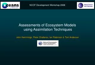
NCOF Development Workshop 2008. Assessments of Ecosystem Models using Assimilation Techniques. John Hemmings, Peter Challenor, Ian Robinson & Tom Anderson. What is the “Ecosystem Model” in Ecosystem Model Assessment ?. Ocean Biogeochemical General Circulation Model. Free-running model

NCOF Development Workshop 2008
E N D
Presentation Transcript
NCOF Development Workshop 2008 Assessments of Ecosystem Models using Assimilation Techniques John Hemmings, Peter Challenor, Ian Robinson & Tom Anderson
What is the “Ecosystem Model” in Ecosystem Model Assessment ? Ocean Biogeochemical General Circulation Model • Free-running model • Assimilation system (sequential D.A.) Ecosystem Sub-model • Fixed parameter model • Model structure and formulation
Outline • The Calibration Process (Inverse D.A. Scheme) • Allowing for Uncertainty • Assessment of D.A. Scheme and Model • Combining Data from Different Locations • Sequential Assimilation of Ocean Colour • Improving Forecasts and Hindcasts
Validation Obs. Sensitivity Analysis OPTIMIZER The Calibration Process Initial Conditions Forcing Boundary Conditions Calibration Obs. ECO. MODEL COST FUNC. Free Parameters Simulated Obs. Science Output Misfit Cost
(xSIM - xOBS)2 2DEP For a given parameter set, 2SIM is uncertainty due to IC, physical forcing & boundary fluxes Allowing for Uncertainty The Misfit Formulation Misfit = 2DEP = 2OBS + 2SIM Estimate 2SIM by: Characterizing uncertainty in IC, physical forcing & boundary fluxes Propagating through model by ensemble runs
Allowing for Uncertainty External Input Data for 1-D Simulations Initial conditions: • Biogeochemical tracer profiles Bi (z, member) Forcing data: • Sea-surface PAR I (t, member) • Sea-surface salinity S (t, member) • Mixed layer depth M (t, member) • Temperature T (z, t, member) • Vertical diffusion coefficient k (z, t, member) • Vertical velocity w (z ,t, member) Boundary fluxes: • Horizontal biogeochemical tracer fluxes Hi (z, t, member)
INPUT ITEMS (1 or more instances of each) free parameters (prior) MODEL SPECIFIC observations N SITES physical forcing Model Evaluator (1-D) N SITES initial conditions N SITES boundary conditions N SITES run options: ecosystem model, time-step, misfit spec. … free parameters (posterior) MODEL SPECIFIC model output fixed parameters M CASES MODEL SPECIFIC Allowing for Uncertainty Marine Model Optimization Test-bed (MarMOT) case table Generic Function Analyzer Optimizer misfit cost misfit cost other validation stats.
REAL-WORLD EXPERIMENTS TWIN EXPERIMENTS • True solution known • Can test parameter recovery + • Ecosystem is real • Uncertainty in IC, forcing, horizontal fluxes and observations affects validation misfit • Idealized scenario may be unrepresentative - Assessment Criteria Assimilation Scheme & Calibration Data Set • No. of parameters constrained (with acceptable repeatability) • Fit to data from non-calibration years - better than prior parameter set
Assessment Criteria Ecosystem Model Calibrated Model: • Fit to data from non-calibration years - better than cal. data climatology Model Structure and Formulation: • Fit to data from non-calibration years • better than alternative model with same cal. data Limitation: optimal calibration not possible for complex models
Ecosystem Model Assessment An Example Model Comparison Experiment OG99 NPZD: Oschlies and Garçon (1999) HadOCC NPZD: Hadley Centre Ocean Carbon Cycle Model, Palmer and Totterdell (2001) - modified Thanks to Ben Ward & Andrew Yool for providing OCCAM output at BATS
Combining Data from Different Locations Identifying Calibration Provinces Zero-D NPZ model fit to daily chlorophyll + winter nitrate at calibration stations Split-domain calibration method (Hemmings, Srokosz, Challenor & Fasham, 2004): identifies optimal geographic ranges for single parameter sets by selecting promising stations to aggregate Final provinces chosen by misfit cost at validation stations NERC Data Assimilation Thematic Programme
3D analysis Observations ΔN Δalk N:Chl 2D analysis of log(Chl) 2D analysis of P Model forecast ΔP ΔZ ΔDIC ΔD Sequential Assimilation of Ocean Colour CASIX Chlorophyll Assimilation Scheme in FOAM-HadOCC DAILY ANALYSIS CYCLE Rosa Barciela, Matt Martin, Mike Bell, Adrian Hines (Met Office) John Hemmings (NOCS) • Aim: improve air-sea CO2 flux by improving surface DIC and alkalinity, hence pCO2 • 2-D analysis of log10(Chl) uses FOAM analysis correction scheme (as for SST) • Surface phytoplankton increments derived using model nitrogen:chl (dynamic) • Other variables adjusted by a new material balancing scheme (Hemmings, Barciela & Bell, 2008)
Sequential Assimilation of Ocean Colour Material Balancing Scheme for Nitrogen and Carbon • Surface phytoplankton increment given as input • Relative increments to other nitrogen pools depend on the likely contributions to phytoplankton error from growth and loss • Nitrogen conserved at each grid point (if possible) • DIC increment conserves carbon • Sub-surface scheme prevents formation of unrealistic sub-surface minima in DIN
Sequential Assimilation of Ocean Colour Evaluation of Material Balancing in 1-D Twin Experiments Assimilating Chl & P 60ºN 50ºN Assimilating Chl only 40ºN 30ºN Free run
DIN physics DA on DA off physics DA on DA off Chlorophyll Sequential Assimilation of Ocean Colour 3-D Evaluation of Chlorophyll Assimilation Scheme TWIN EXPERIMENTS REAL-WORLD EXPERIMENTS Surface Chlorophyll Un-assimilated Variables ? Biogeochemical errors due to excessive vertical transport of nutrients not corrected by chlorophyll assimilation (intentionally) Impact of Physical D.A. (link to MARQUEST) Need biogeochemical balancing scheme when assimilating T&S profiles
Improving Forecasts and Hindcasts: the Role of Parameter Optimization A Non-identical Twin Experiment Truth: HadOCC Ecosystem Model: Simplified HadOCC with 4 free parameters Calibration data: Chlorophyll (daily), DIN & pCO2 (monthly)
Improving Forecasts and Hindcasts: the Role of Parameter Optimization Sequential Chlorophyll Assimilation Results Surface Chlorophyll TRUTH Surface Phytoplankton ORIGINAL ORIGINAL + CHL D.A. Surface DIN OPTIMIZED OPTIMIZED + CHL D.A. Surface pCO2
Improving Forecasts and Hindcasts Application of Different Assimilation Methods Sequential Data Assimilation • Improve hindcast state • Improve initial conditions for short-term forecasts Parameter Optimization (Inverse D.A. Methods) • Improve long-term forecast • Improve performance of sequential schemes