Download
1 / 37
400 likes | 696 Views
Graph Theory vs The Curse of Dimensionality. Matt Smith PhD Banner Health Analytics & Innovation. Health Care Data. What’s on my chart?. ICD-10 Codes. ICD-10 Codes record the details of your health care encounter They are used to standardize record keeping and billing

E N D
Graph TheoryvsThe Curse of Dimensionality Matt Smith PhD Banner Health Analytics & Innovation
Health Care Data What’s on my chart?
ICD-10 Codes • ICD-10 Codes record the details of your health care encounter • They are used to standardize record keeping and billing • There are codes for different aspects of why you are in contact with a health care provider • Is there a specific disease? • A traumatic event? • Where did it happen? • Are there any complications?
Encounter Records • If a medical provider takes notes:27 year old female, with medical history of [redacted] with prior diagnosis of [redacted], who presented with right shoulder [redacted], admitted for right shoulder cellulitis and fascitis and concerns for abscess. • Records would show:
ICD-10 Codes (Formally) • The International Classification of Diseases (ICD) is the international standard diagnostic tool for epidemiology, health management, and clinical purposes. • Created and maintained by the World Health Organization • ICD-10 is the 10th version • Developed between 1983 and 1990 • Used in 27 countries • Adopted in US in early 2000’s (completed in 2015)
ICD-10 Organization • ICD-10 codes are structured • The leading entry and modifier are letters • All other entries are 0-9. Modifier Category Vital Details
There’s a lot of codes • There are about 70,000 codes • This number depends on who you ask. It can vary based on criteria such as billable/non-billable status. • The structure of the codes is the main reason the number is so high
Data and Dimensions Too many variables is a problem.
Dimensions in Data • We can think of the typical dataset as a grid with rows and columns • The rows are usually called observations or datapoints • The columns are usually called variables or dimensions
A Curse of Dimensionality • If we have a lot of dimensions, almost observation is an outlier • Assuming we have independent variables • Also assume we have a “nice” distribution • Define outliers as observations with values in the lowest or highest 2.5% of values for at least one dimension • For 1 dimension, 5% of observations are outliers. • For 5 dimensions, 23% of observations are outliers. • For 10 dimensions, 40% of observations are outliers. • For 50 dimensions, 92% of observations are outliers.
Diagnosis codes are a lot of dimensions • Encounters and diagnoses give us a big data set • For a given encounter, each ICD code is a variable • 1 = Diagnosis applies, 0 = Otherwise • Encounters frequently have rare codes • The condition might not be rare, but code specificity makes it look rare
Dimension Reduction • Reducing the number of dimensions solves most the problems stemming from the curse of dimensionality • Select a subset of variables • Map variables to a smaller set of new variables • Popular methods • Principle Component Analysis • Manifold Embedding • Neutral Net-based Autoencoding
But … • Most popular methods only work when specific assumptions are met • Most require variables to be continuous • Some have distribution assumptions • ICD codes are discrete (1 = Diagnosis applies, 0 = Otherwise) • Output from autoencoders is difficult for humans to interpret
Networks The friendly name for Graph Theory
Graphs • A graph is a set with connections between members of that set.
Graph Terminology • The points are usually called vertices or nodes • The connections are usually called edges • The edges are individually assigned numeric values called weights. • For our purposes the weights are positive real numbers • We use higher real values to represent stronger connections between nodes
Linear Algebra & Networks It’s move than solving Ax = b.
Adjacency Matrices • For a graph with nnodes, the adjacency matrixA of the graph is an matrix with equal to the weight of the edge between nodes iand j (this is 0 if there is no edge). 3 1 5 4 2 6
Degree Matrices • For a graph with nnodes, the degree matrixD of the graph is an matrix with equal to the sum of weights connecting node i to all other nodes. All other entries are 0. 3 1 5 4 2 6
Laplacian Matrices • There Laplacianmatrix Lof a graph is D – A. • Maybe named from modeling change in heat distribution on a graph. The Laplacian matrix takes the place of the Lacplacian operator in the heat model. 3 1 5 4 2 6
Graphs and Dimensions • Think of the nodes as diagnoses • The edge weights between a pair of diagnoses are how many encounters that pair of the diagnoses appear together • We will map this graph to Rk for a “small” value of k • We can think of diagnoses as points in Rk rather 1 of 70,000 possible values! • We want highly connected nodes to be close together and unconnected nodes to be far apart
Graph Mapping and the Laplacian • Suppose we have a graph with n nodes and its LacplacianL • We think of vector x as a mapping of the graph’s nodes to points in R • xi is the location of node i • If we conjugate L by x we have xTLx = ∑ aij (xi – xj)2 • If we are buying edges by the inch, xTLx shows the cost of using mapping x • We are looking for a low cost mapping
“Low Cost” Graph Mapping • This quantity is minimized when x = [1, 1, … , 1] T • In this case xTLx = 0 • But this isn’t a useful mapping – all the nodes are on the same place! • We can find low values for xTLxwith some reasonable constraints
Eigenvalues of the Laplacian • We will assume our graph is fully connected • If we start on an arbitrary node, we can reach every other node by walking along the edges • L is a positive semidefinite real symmetric matrix • The eigenvalues are non-negative real numbers • The eigenvectors corresponded to distinct eigenvalues are orthogonal • Let the eigenvalues of Lbe 0 = λ1 < λ2 ≤ λ3 ≤ … ≤ λnwith corresponding eigenvectors v1, v2, v3, … , n
Rayleigh – Ritz Theorem • When x is a unit vector, xTLxis the Rayleigh quotient for L • From now on, all vectors are unit vectors • Note that viTLvi= λi • A consequence of the Rayleigh-Ritz theorem tells us the minimum value of xTLx where x is orthogonal to [1, 1, … , 1] Tiswhen x is an eigenvector corresponding to λ2 • Orthogonality to the constant vector while minimizing the Rayleigh quotient means that heavily connected groups of vertices stay close together but aren’t mapped right on top of each other
Graph Mapping – Multidimensional • We can build a low cost mapping using eigenvectors corresponding the smallest eigenvalues • Define M to be an nk matrix where the i-th column is vi+1 • The columns are orthogonal and normal • Maps the graph into Rk • The “cost” of the mapping is λ2 +λ3+ … + λk+1 • This is optimal if we want an orthogonal group of vectors that keep connected nodes close but don’t map all the vertices to the same spot • Some other conditions apply … but we won’t worry about that
Rayleigh – Ritz Theorem (again) • As the eigenvalues grow, our mapping gets more expensive • xTLx achieves its highest values for vn - eigenvectors corresponding to the largest eigenvalue • Because we are reducing dimensions, we want k to be much smaller than n • As long as we use eigenvectors associated with small eigenvalues, our mapping will keep strongly connected nodes close together
Laplacian Matrices – Different Flavors • The spectrum of L is heavily dependent on the degree distribution of the graph • There are two popular derivatives of the Laplacian that use normalization to prevent this • The symmetric normalized Laplacianis D-1/2LD-1/2 • The random walk Laplacianis D-1L • These definitions are not universal! Different sources will have different versions
Results So, did this actually work?
BTW … • This is section is limited • There are concerns about information recovered from a mapping • Not patient-level detail, but overall information about the health condition of our patient population • Mappings and models based on them are proprietary information
Building the Graph • We built a diagnosis graph • The nodes are ICD codes • The edges are weighted as follows: • For each encounter, take the list of ICD codes • If codes i and j are in the list, add 1 to the weight of edge between them
Building the Graph I12.9 • *This isn’t the whole story. We considered diagnostic priority when adding weight. And we might have “smoothed” the degree distribution. R21 I19 A41.9 C79.31 C79.32 J18.0
Eigenvalues of the Graph Laplacian • We used normalized versions of the Laplacian • We used 8 eigenvectors for the mapping • Different vectors separate different aspects • One cluster of tightly connected diagnoses mapped to one end of an eigenvector and the rest mapped to the other
Interesting Results • Vectors associated with the smallest eigenvalues separate pregnancy related diagnoses • Vectors associated with the middle eigenvalues separate bodily systems • Circulatory, Respiratory, Etc. • Vectors associated with the larger eigenvalues separate emergency and trauma causes
References Wait – that didn’t make sense!
References • General Graph Theory • D. West, Introduction to Graph Theory • A. Bondy & U. S. R. Murty, Graph Theory with Applications • Longer Spectral Graph Theory Texts • F. Chung, Spectral Graph Theory • http://www.math.ucsd.edu/~fan/ • M. W. Mahoney, Lecture Notes on Spectral Graph Methods • arXiv:1608.04845v1 • D. Spielman, Lecture notes • http://www.cs.yale.edu/homes/spielman/561/ • Shorter Spectral Graph Theory Documents • U. von Luxburg, A Tutorial on Spectral Clustering • arXiv:0711.0189v1 • C. Jiang, Introduction to Spectral Graph Theory and Graph Clustering • http://web.cs.ucdavis.edu/~bai/ECS231/ho_clustering.pdf • J. Gallier, Notes on Elementary Spectral Graph Theory Applications to Graph Clustering Using Normalized Cuts • arXiv:1311.2492