Download
1 / 32
320 likes | 430 Views
Eigenpattern Analysis of Geophysical Data Sets Applications to Southern California. K. Tiampo, University of Colorado with J.B. Rundle, University of Colorado S. McGinnis, University of Colorado W. Klein, LANL & Boston University. Work funded under NASA Grant NAG5-9448. Abstract.

E N D
Eigenpattern Analysis of Geophysical Data Sets Applications to Southern California K. Tiampo, University of Colorado with J.B. Rundle, University of Colorado S. McGinnis, University of Colorado W. Klein, LANL & Boston University Work funded under NASA Grant NAG5-9448
Abstract Earthquake fault systems are now thought to be an example of a complex nonlinear system (Bak, 1987; Rundle, 1995). Under the influence of a persistent driving force, the plate motions, interactions among a spatial network of fault segments are mediated by means of a potential that allows stresses to be redistributed to other segments following slip on another segment. The slipping segment can trigger slip at other locations on the fault surface whose stress levels are near the failure threshold as the event begins. In this manner, earthquakes occur that result from the interactions and nonlinear nature of the stress thresholds. This spatial and temporal system complexity translates into a similar complexity in the surface expression of the underlying physics, including deformation and seismicity. Specifically, the southern California fault system demonstrates complex space-time patterns in seismicity that include repetitive events, precursory activity and quiescience, as well as aftershock sequences. Our research suggests that a new pattern dynamic methodology can be used to define a unique, finite set of seismicity patterns for a given fault system (Tiampo et al., 2002). Similar in nature to the empirical orthogonal functions historically employed in the analysis of atmospheric and oceanographic phenomena (Preisendorfer, 1988), the method derives the eigenvalues and eigenstates from the diagonalization of the correlation matrix using a Karhunen-Loeve expansion (Fukunaga, 1990, Rundle, et al., 1999). This Karhunen-Loeve expansion (KLE) technique may be used to help determine the important modes in both time and space for southern California seismicity as well as deformation (GPS) data. These modes potentially include such time dependent signals as plate velocities, viscoelasticity, and seasonal effects. This can be used to better model geophysical signals of interest such as coseismic deformation, viscoelastic effects, and creep. These, in turn, can be used for both model verification in large-scale numerical simulations of southern California and error analysis of remote sensing techniques such as InSar.
Background • Earthquakes are a high dimensional complex system having many scales in space and time. • New approaches based on computational physics, information technology, and nonlinear dynamics of high-dimensional complex systems suggest that earthquakes faults are strongly correlated systems whose dynamics are strongly coupled across all scales. • The appearance of scaling relations such as the Gutenberg-Richter and Omori laws implies that earthquake seismicity is associated with strongly correlated dynamics, where major earthquakes occur if the stress on a fault is spatially coherent and correlated near the failure threshold. • Simulations show that regions of spatially coherent stress are associated with spatially coherent regions of anomalous seismicity (quiescence or activation). • The space-time patterns that earthquakes display can be understood using correlation-operator analysis (Karhunen-Loeve, Principal Component, etc.). • Studies of the pattern dynamics of space-time earthquake patterns suggests that an understanding of the underlying process is possible.
Time Series Analysis Overview • Surface deformation and seismicity are the surface expression of the underlying fault system dynamics. • Time series analysis of various types can illuminate particular features or signals in the data. • We will begin with an overview of the modeling that prompted this analysis. • We will the follow with three applications: - Karhunen-Loeve (KL) decomposition of GPS deformation into its eigenpatterns. - KL decomposition of historic seismicity for southern California into its eigenpatterns. - Pattern dynamics analysis of the same seismic data set.
Fault System Basics Leaky Threshold F Dynamics of an isolated cell R Cell State F Threshold R Time A high dimensional complex system with many identical, connected (interacting) units or cells, and thus many degrees of freedom. In many such systems, each cell has an internal state variable that cycles between a low (residual) value R and a high (threshold) value F. In the case of faults, this variable is stress. In a driven threshold system, the value of is driven persistently upward through time from R towards F as a result of external forcings. When the condition = F is satisfied, the cell becomes unstable, at which time the state decreases suddenly to R. In a leaky threshold system, a process exists that allows some of the state to “leak away” from the cell at a rate that depends inversely on the value of - R.
Fault Network Model The stress on a fault patch is controlled by the frictional strength of the patch, as governed by its coefficient of friction. At right is the result of the calculation of S - K for the Virtual_California 2000 model. This difference in friction coefficients determines the nominal values of slip on the various fault segments.
Surface Deformation from Earthquakes There is a wealth of data characterizing the surface deformation observed following earthquakes. As an example, we show data from the October 16, 1999 Hector Mine event in the Mojave Desert of California. At left is a map of the surface rupture. Below is the surface displacement observed via GPS (right) and via Synthetic Aperature Radar Interferometry (JPL), and InSAR (JPL) (below).
Simulated Pre- vs. Post- Seismic Displacements: GPS( LEFT: Pre-seismic 5 years; RIGHT: Post-seismic 5 years )
Pre- vs. Post- Without Earthquakes: InSAR - C( LEFT: Pre-seismic 5 years; RIGHT: Post-seismic 5 years) The difference fringes are small (red = positive and blue = negative regions), and are concentrated along the portions of the San Andreas that are about to initiate sliding (the asperities). The amplitude of the difference red - blue is about 1/2 fringe or ~ 3 CM
Karhunen-Loeve Analysis • A Karhunen-Loeve (KL) expansion analysis is a method for decomposing large data sets into their orthonormal eigenvectors and associated time series, based upon the correlations that exist in the data. • The vector space is spanned by the eigenvectors, or eigenpatterns, of an N-dimensional, KL correlation matrix, C(xi,xj). The elements of C are obtained by cross-correlating a set of location time series. • The eigenvalues and eigenvectors of C are computed using a standard decomposition technique, producing a complete, orthonormal set of basis vectors which represent the correlations in the seismicity data in space and time. • This method can be used to study those modes most responsible for these correlations and their sources (Savage, 1988), to remove those uninteresting modes in the system (Preisendorfer, 1988), or project their trajectories forward in time (Penland and others). Here we begin with deformation in southern California.
Southern California Integrated GPS Network (SCIGN) • The first stations were installed in 1991. Today there are over 200 stations throughout southern California. • Two different data analyses methods, SCIGN 1.0 and 2.0. • SCIGN 1.0 has repeatabilities of 3.7 mm latitude, 5.5 mm longitude, and 10.3 mm vertical. • SCIGN 2.0 has repeatabilities of 1.2 mm latitude, 1.3 mm longitude, and 4.4 mm vertical.
Sample Data, SCIGN 1.0 and 2.0 JPLM AOA1
Decomposition • We broke the decompositions down into pre- and post-1998. • The KLE method was applied to both the SCIGN 1.0 vertical data and the latitude-longitude (horizontal) data, for the time period 1993-1997, inclusive. • Analysis of the data beginning 1 January, 1998, included only the SCIGN 2.0 data, ending in mid-2000. • This same analysis, pre- and post-1998, vertical and horizontal, was performed for both the entire data set, consisting of approximately 200 stations in 2000, and just the LA basin.
First Horizontal KL Mode - Velocity SCIGN 1.0, All Data SOPAC/JPL Velocity Model
First Horizontal KL Mode - Velocity SCIGN 2.0, LA Basin SOPAC/JPL Velocity Model
SCIGN 1.0, Horizontal Mode 4 - Deformation Following the 1994 Northridge Earthquake (Donnellan & Lyzenga, 1998)
SCIGN 1.0, First KL Vertical Mode (Susanna Gross, unpublished)
SCIGN 2.0, KL Mode 2 – Hector Mine All Stations LA Basin Vertical Vertical Horizontal Horizontal
Seismicity Data • Southern California Earthquake Center (SCEC) earthquake catalog for the period 1932-1999. • Data for analysis: 1932-1999, M ≥ 3.0. • Events are binned into areas 0.1° to a side (approximately 11 kms), over an area ranging from 32° to 39° latitude, -122° to -115° longitude. • A matrix is created consisting of the daily seismicity time series (n time steps) for each location (p locations). • This data matrix is cross-correlated in the KL decomposition.
Correlated Patterns in Computer Simulations: Activity Eigenpatterns 1 – 4
Correlated Patterns in Historic Seismicity Data Karhunen-Loeve Decomposition, 1932-1998
Southern California Seismicity, 1932 through 1991 KLE2 KLE1 Note: Landers, M7.1, occurs in 1992
1932 through 1991 KLE8 KLE4 KLE17
EIGENVALUE POWER, 1991 EIGENVALUE POWER, 1990 EIGENVALUE POWER, 1989 Decomposition of Annual Seismicity into Individual KLE modes 8 17 Mode
Phase Dynamical Probability Change (PDPC) Index • We have developed a method called phase dynamics to the seismicity data, in order to detect changes in observable seismicity prior to major earthquakes, via the temporal development of spatially coherent regions of seismicity. • The PDPC index is computed directly from seismicity data, but is based upon the idea that earthquakes are a strongly correlated dynamical system, similar to neural networks, superconductors, and turbulence. Various features of these systems can be described using phase dynamics. • Define a phase function = / , where is a nonlocal function, incorporating information from the entire spatial domain of x, including spatial patterns, correlations and coherent structures. • is a vector that moves in random walk increments on a unit sphere in N-dimensional space. Seismicity is interpreted as a phase dynamical system, in which the dynamic evolution of the system corresponds to the rotation of . • The probability change, or the PDPC, for the formation of a coherent seismicity structure is then
Southern California Seismicity, 1932-1991 • This map shows the intensity of seismicity in Southern California during the period 1932-1991, normalized to the maximum value. • Most intense red areas are regions of most intense seismic activity.
PDPC Anomalies, S. California, 1978-1991: Actual (left) and Random (right) Catalogs
Anomalous Seismic Activity Patterns • Does the PDPC method detect anomalous activity or anomalous quiescence? Both. • On the right is shown the corresponding patterns of anomalous activity (red) and anomalous quiescence (blue) during 1978-1991.
Anomalous Seismic Moment ReleaseCase 1: Hidden Structures Bawden, Michael and Kellogg, Geology, 1999
Anomalous Seismic Moment Release Case 2: Aseismic slip without radiated seismic waves. Unwrapped interferogram, 1992 to 1997 Courtesy P. Vincent, LLNL.
Anomalous Seismic Moment Release Case 3: Forecasting PDPC Index 10 years prior to: Imperial Valley, 1979 Loma Prieta, 1989
Conclusions • Earthquake fault systems are characterized by strongly correlated dynamics, implying the existence of space-time patterns and scaling distributions. • Both standard and unconventional methods of time series analysis can be used to identify the eigenpatterns of the surface expression of these underlying correlations. • Earthquake fault systems can evidently be considered to be an example of a phase dynamical system, implying that the important changes are represented by rotations of phase functions in a high-dimensional correlation space. • This phase dynamical interpretation can be used to locate areas of actual and potential seismic moment release for the purposes of identifying underlying features of the fault system.