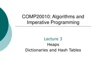
COMP20010: Algorithms and Imperative Programming
COMP20010: Algorithms and Imperative Programming. Lecture 2 Data structures for binary trees Priority queues. Lecture outline. Different data structures for representing binary trees (vector-based, linked), linked structure for general trees; Priority queues (PQs), sorting using PQs;.

COMP20010: Algorithms and Imperative Programming
E N D
Presentation Transcript
COMP20010: Algorithms and Imperative Programming Lecture 2 Data structures for binary trees Priority queues
Lecture outline • Different data structures for representing binary trees (vector-based, linked), linked structure for general trees; • Priority queues (PQs), sorting using PQs;
A vector-based structure for binary trees is based on a simple way of numbering the nodes of T. For every node v of T define an integer p(v): If v is the root, then p(v)=1; If v is the left child of the node u, then p(v)=2p(u); If v is the right child of the node u, then p(v)=2p(u)+1; The numbering function p(.) is known as a level numbering of the nodes in a binary tree T. Data structures for representing treesA vector-based data structure
Data structures for representing treesA vector-based data structure • ((((3+1)*3)/((9-5)+2))-((3*(7-4))+6)) 1 - 3 2 + / 7 5 6 4 * 6 + * 13 9 10 11 12 8 14 15 - + 3 - 2 3 27 26 16 17 20 21 18 19 9 5 22 23 24 25 7 4 3 1 Binary tree level numbering
Data structures for representing treesA vector-based data structure • The level numbering suggests a representation of a binary tree T by a vector S, such that the node v from T is associated with an element S[p(v)]; 1 - 3 2 + / 7 5 6 4 * 6 + * 13 9 10 11 12 8 14 15 - + 3 - 2 3 27 26 16 17 20 21 18 19 9 5 22 23 24 25 7 4 3 1 S - / + * + * 6 + 3 - 2 3 - 3 1 9 5 7 4
Data structures for representing treesA vector-based data structure Running times of the methods when a binary tree T is implemented as a vector
Data structures for representing treesA linked data structure • The vector implementation of a binary tree is fast and simple, but it may be space inefficient when the tree height is large (why?); • A natural way of representing a binary tree is to use a linked structure. • Each node of T is represented by an object that references to the element v and the positions associated with with its parent and children. parent element left child right child
Data structures for representing treesA linked data structure for binary trees null A A C C B B null null E D E D null null F G F G null null null null
Data structures for representing treesA linked data structure for general trees • In order to extend the previous data structure to the case of general trees; • In order to register a potentially large number of children of a node, we need to use a container (a list or a vector) to store the children, instead of using instance variables; null A A B C D E C D E B null null null null
Keys and the total order relation • In various applications it is frequently required to compare and rank objects according to some parameters or properties, called keys that are assigned to each object in a collection. • A key is an object assigned to an element as a specific attribute that can be used to identify, rank or weight that element. • A rule for comparing keys needs to be robustly defined (not contradicting). • We need to define a total order relation, denoted by with the following properties: • Reflexive property: ; • Antisymmetric property: if and , then ; • Transitive property: if and , then ; • The comparison rule that satisfies the above properties defines a linear ordering relationship among a set of keys. • In a finite collection of elements with a defined total order relation we can define the smallest key as the key for which for any other key k in the collection.
Priority queues • A priority queueP is a container of elements with keys associated to them at the time of insertion. • Two fundamental methods of a priority queue P are: • insertItem(k,e) – inserts an element e with a key k into P; • removeMin() – returns and removes from P an element with a smallest key; • The priority queue ADT is simpler than that of the sequence ADT. This simplicity originates from the fact that the elements in a PQ are inserted and removed based on their keys, while the elements are inserted and removed from a sequence based on their positions and ranks.
Priority queues • A comparator is an object that compares two keys. It is associated with a priority queue at the time of construction. • A comparator method provides the following objects, each taking two keys and comparing them: • isLess( ) – true if ; • isLessOrEqualTo( ) – true if ; • isEqualTo( ) – true if ; • isGreater( ) – true if ; • isGreaterOrEqualTo( ) – true if ; • isComparable(k) – true if k can be compared;
PQ-Sort • Sorting problem is to transform a collection C of n elements that can be compared and ordered according to a total order relation. • Algorithm outline: • Given a collection C of n elements; • In the first phase we put the elements of C into an initially empty priority queue P by applying n insertItem(c) operations; • In the second phase we extract the elements from P in non-decreasing order by applying n removeMinoperations, and putting them back into C;
PQ-Sort • Algorithm PQ-Sort(C,P); • Input: A sequence C[1:n] and a priority queue P that compares keys (elements of C) using a total order relation; • Output: A sequence C[1:n] sorted by the total order relation; whileC is not empty do e C.removeFirst(); {remove an element e from C} P.insertItem(e,e); {the key is the element itself} while P is not empty do e P.removeMin() {remove the smallest element from P} C.insertLast(e) {add the element at the end of C} • This algorithm does not specify how the priority queue P is implemented. Depending on that, several popular schemes can be obtained, such as selection-sort, insertion-sort and heap-sort.
Priority queue implemented with an unordered sequence and Selection-Sort • Assume that the elements of P and their keys are stored in a sequence S, which is implemented as either an array or a doubly-linked list. • The elements of S are pairs (k,e), where e is an element of P and k is the key. • New element is added to S by appending it at the end (executing insertLast(k,e)), which means that S will be unsorted. • insertLast() will take O(1) time, but finding the element in S with a minimal key will take O(n).
Priority queue implemented with an unordered sequence and Selection-Sort • The first phase of the algorithm takes O(n) time, assuming that each insertion takes O(1) time. • Assuming that two keys can be compared in O(1) time, the execution time of each removeMin operation is proportional to the number of elements currently in P. • The main bottleneck of this algorithm is the repeated selection of a minimal element from an unsorted sequence in Phase 2. This is why the algorithm is referred to as selection-sort. • The bottleneck of the selection-sort algorithm is the second phase. Total time needed for the second phase is
Priority queue implemented with a sorted sequence and Insertion-Sort • An alternative approach is to sort the elements in the sequence S by their key values. • In this case the method removeMin actually removes the first element from S, which takes O(1) time. • However, the method insertItem requires to scan through the sequence S for an appropriate position to insert the new element and its key. This takes O(n) time. • The main bottleneck of this algorithm is the repeated insertion of elements into a sorted priority queue. This is why the algorithm is referred to as insertion-sort. • The total execution time of insertion-sort is dominated by the first phase and is .