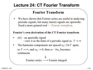
Lecture 24: CT Fourier Transform
Lecture 24: CT Fourier Transform. Symmetry Property: Example. Property of Duality. Illustration of the duality property. More Properties. Example: Fourier Transform of a Step Signal. Lets calculate the Fourier transform X ( j w )of x ( t ) = u ( t ), making use of the knowledge that:

Lecture 24: CT Fourier Transform
E N D
Presentation Transcript
Example: Fourier Transform of a Step Signal • Lets calculate the Fourier transform X(jw)of x(t) = u(t), making use of the knowledge that: • and noting that: • Taking Fourier transform of both sides • using the integration property. Since G(jw) = 1: • We can also apply the differentiation property in reverse
Proof of Convolution Property • Taking Fourier transforms gives: • Interchanging the order of integration, we have • By the time shift property, the bracketed term is e-jwtH(jw), so
Convolution in the Frequency Domain • To solve for the differential/convolution equation using Fourier transforms: • Calculate Fourier transforms of x(t) and h(t) • Multiply H(jw) by X(jw) to obtain Y(jw) • Calculate the inverse Fourier transform of Y(jw) • Multiplication in the frequency domain corresponds to convolution in the time domain and vice versa.
Example 1: Solving an ODE • Consider the LTI system time impulse response • to the input signal • Transforming these signals into the frequency domain • and the frequency response is • to convert this to the time domain, express as partial fractions: • Therefore, the time domain response is: ba
H(jw) -wc wc w Example 2: Designing a Low Pass Filter • Lets design a low pass filter: • The impulse response of this filter is the inverse Fourier transform • which is an ideal low pass filter • Non-causal (how to build) • The time-domain oscillations may be undesirable • How to approximate the frequency selection characteristics? • Consider the system with impulse response: • Causal and non-oscillatory time domain response and performs a degree of low pass filtering
Lecture 27: Summary • The Fourier transform is widely used for designing filters. You can design systems which reject high frequency noise and just retain the low frequency components. This is natural to describe in the frequency domain. • Important properties of the Fourier transform are: • 1. Linearity and time shifts • 2. Differentiation • 3. Convolution • Some operations are simplified in the frequency domain, but there are a number of signals for which the Fourier transform do not exist – this leads naturally onto Laplace transforms