Download

1 / 46
460 likes | 707 Views
Spreadsheet-Based Decision Support Systems. Chapter 19: The Solver Re-Visited. Prof. Name name@email.com Position (123) 456-7890 University Name. Overview. 19.1 Introduction 19.2 Review of Chapter 8 19.3 Solver commands in VBA

E N D
Spreadsheet-Based Decision Support Systems Chapter 19: The Solver Re-Visited Prof. Name name@email.com Position (123) 456-7890 University Name
Overview • 19.1 Introduction • 19.2 Review of Chapter 8 • 19.3 Solver commands in VBA • 19.4 Application • 19.5 Summary
Introduction • Preparing an optimization problem to be solved by the Solver • Preparing and running the Solver using VBA functions • A dynamic optimization application using VBA Solver functions
Review of Chapter 8 • Understanding the problem • Preparing the spreadsheet • Solving the Model
Review of Chapter 8 • In Chapter 8 we described how to transform a problem into a mathematical model and then use the Excel Solver to solve it. • We will review the main parts of a mathematical model and the Solver preparation steps. • There are important steps which take place in the Excel spreadsheet before the Solver is used. • Reading and Interpreting the Problem • Preparing the Spreadsheet
Understanding the Problem • Mathematical models transform a word problem into a set of equations that clearly define the values you are seeking given the limitations of the problem. • There are three main parts of a mathematical model. • Decision variables • Objective function • Constraints
Decision Variables • Decision variables are variables that are assigned to a quantity or response that you must determine in the problem. • They can be defined as negative, non-negative, or unrestricted variables. • An unrestricted variable can be either negative or non-negative. • These variables are used to represent all other relationships in the model, including the objective function and constraints.
Objective Function • The objective function is an equation that states the goal, or objective, of the model. • Objective functions are either maximized or minimized. • Most applications involve maximizing profit or minimizing cost.
Constraints • The constraints are the limitations of the problem. • In most realistic problems there are certain limitations, or constraints, which we must consider. • Constraints can be a limited amount of resources, labor, or requirements for a particular demand. • These constraints are also written as equations in terms of the decision variables.
Applying a model • In understanding the problem, we define the mathematical model. • That is, we must define our decision variables, objective function, and constraints via mathematical representation. • We saw some examples in Chapter 8 which involved production of different parts. • The amount to produce of each part was considered the decision variables. • Maximizing profit (given certain costs and revenues for each part was the objective function. • There were also constraints which limited the resources needed for each part and stated a minimum demand that had to be met.
Preparing the Worksheet • We must translate and clearly define each part of our model in the spreadsheet. • The Solver will then interpret our model according to how we have declared the decision variables, objective function, and constraints in the spreadsheet. • We use referencing and formulas to mathematically represent the model in the spreadsheet cells.
Entering Decision Variables • To enter the decision variables, we list them in individual cells with an empty cell next to each one. • The Solver will place values in these cells for each decision variable as it solves the model. • All other equations (for the objective function and constraints) will reference these cells.
Entering Objective Function • To enter the objective function, we place our objective function equation in a cell with an adjacent description. • This equation should be entered as a formula which references the decision variable cells. • As the Solver changes the decision variable values in the decision variable cells, the objective function value will automatically be updated.
Entering Constraints • To enter the constraints we list the equations separately with a description next to each constraint. • The most important part of setting up the constraint table is expressing the left side of our equations as formulas. • As each constraint is in terms of the decision variables, all of these formulas must be in terms of the decision variable cells that Solver uses. • These equations should reference the decision variable cells so that as the Solver places values in these cells the constraint values will automatically be calculated. • Another important consideration when laying out the constraints in preparation for Solver is that the RHS (right-hand side) values of each constraint should be in individual cells to the right of these equations. • We should also place all inequality signs in their own cells.
Naming the Ranges • Another advantageous way to keep our constraints organized as we use the Solver is to name our cells. • Using the methods discussed in Chapter 3, we can name the ranges decision variables and the cell which holds the objective function equation. • We can also name ranges of constraint equations which are in a similar category of constraints or which have similar inequality signs. • This makes inserting these model parts into the Solver easier when using both Excel and VBA code .
Solver Example from Chapter 8 • A company produces six different types of products. They want to schedule their production to determine how much of each product type should be produced in order to maximize their profits. This is known as the Product Mix problem. • Production of each product type requires labor and raw materials; but the company is limited by the amount of resources available. • There is also a limited demand for each product, and no more than this demand per product type can be produced. Input tables for the necessary resources and the demand are given.
Step 1 • Decision Variables: The amount produced of each product type. • x1, x2, x3, x4, x5, x6 • Objective Function: Maximize Profit. • z = p1*x1 + p2*x2 + p3*x3 + p4*x4 + p5*x5 + p6*x6 • Constraints: There are two resource constraints: labor, l, and raw material, r. • Labor Constraint: • l1*x1 + l 2*x2 + l 3*x3 + l4*x4 + l 5*x5 + l 6*x6 <= available labor = 4500 • Raw Material Constraint • r1*x1 + r 2*x2 + r 3*x3 + r 4*x4 + r 5*x5 + r 6*x6 <= available raw material = 1600 • There is also a constraint that all demand, D, must be met, and no extra amount can be produced. • Demand Constraint: • xi <= Di for i = 1 to 6
Figure 19.3 • The Results of the Solver are shown • All constraints are met
Solver Commands in VBA • Identifying Solver Input • Setting Solver Options • Running the Solver • Generating Reports
Solver Commands in VBA • We now learn how to identify the ranges which contain the decision variables, objective function, and constraints as input to the Solver using VBA code. • We also learn how to set Solver options and run the Solver in VBA. • We then see what VBA commands will generate Solver reports.
Identifying Solver Input • The SolverOK function is used to set the objective function and decision variables. • SolverOK(SetCell, MaxMinVal, ValueOf, ByChange) • The SetCell argument is used to specify the range of the objective function. • The MaxMinVal argument specifies if this objective function will be maximized, minimized, or solved to a particular value. • 1( = maximize) • 2 (= minimize) • 3 (= value) • If this argument value is 3, then the ValueOf argument is used to set this value. • The ByChange argument specifies the range which contains the decision variables.
Example Input SolverOK SetCell:=Range("F28"), MaxMinVal:=1, ByChange:=Range("E14:E15") • For this example, we had also named the input ranges; therefore, we can instead type the following SolverOK SetCell:=Range("ObjFunc"), MaxMinVal:=1, ByChange:=Range("DecVar")
Identifying Solver Input (cont) • The SolverAdd function should be used to add each individual constraint or each group of similar constraints. • SolverAdd(CellRef, Relation, FormulaText) • The CellRef argument specifies the range which contains a constraint equation. • The Relation argument can take one of five values which specify the inequality of the constraint. • 1 is <= • 2 is = • 3 is >= • 4 is int • 5 is bin • The FormulaText argument specifies the range which contains the RHS value of the constraint.
Example Input (cont) SolverAdd CellRef:=Range(“C18:C20”), Relation:=3, FormulaText:=Range(“F18:F20”) SolverAdd CellRef:=Range(“C21:C23”), Relation:=1, FormulaText:=Range(“F21:F23”) SolverAdd CellRef:=Range(“C24”), Relation:=1, FormulaText:=Range(“F24”) SolverAdd CellRef:=Range(“C25”), Relation:=1, FormulaText:=Range(“F25”) • Again, since we named our constraint ranges, we could have instead typed SolverAdd CellRef:=Range(“QuotaCon”), Relation:=3, FormulaText:=Range(“F18:F20”) SolverAdd CellRef:=Range(“LimitCon”), Relation:=1, FormulaText:=Range(“F21:F23”) SolverAdd CellRef:=Range(“WeightCon”), Relation:=1, FormulaText:=Range(“F24”) SolverAdd CellRef:=Range(“SpaceCon”), Relation:=1, FormulaText:=Range(“F25”)
Identifying Solver Input (cont) • There are two more functions which can be used to modify constraints. • SolverChange and SolverDelete • These functions will allow you to modify or delete a constraints, respectively. • They both have the same arguments as the SolverAdd function. • Another function, which can be used before any input is entered, is the SolverReset function. • This function resets all Solver parameters. • All input will be empty and all Solver options will be set to their default values. • It is generally a good idea to use this function before any of the above input functions are used.
Setting Solver Options • To set the Solver options in VBA, we use the SolverOptions function. • This function has many arguments for each of the options we have seen previously in the Solver Options dialog box. • There are two arguments which we will use more frequently, which are AssumeLinear and AssumeNonNeg. • Both of these arguments take True/False values. • True makes the corresponding assumption. • For most of our models, we will set both of these arguments to true as follows. SolverOptions AssumeLinear:=True, AssumeNonNeg:=True • The other option arguments include: MaxTime, Iterations, Precision, StepThru, Estimates, Derivatives, Search, IntTol, Scaling, and Convergence.
Running the Solver • To run the Solver in VBA, we use the function SolverSolve. • This function has two arguments and is written as follows. SolverSolve(UserFinish, ShowRef) • The UserFinish argument uses a True/False value to determine whether to return the Solver results with our without showing the Solver Results dialog box. • We will usually set this argument value to True. • If the value is False then the Solver Results dialog box will appear after the Solver has run the model. • The ShowRef argument is used when the StepThru option is set; hence we will usually ignore this argument. SolverSolve UserFinish:=True
Solver Solution • The SolverSolve function also returns an integer value classifying the result. • The values 0, 1, or 2 signify a successful run in which a solution has been found. • The value 4 implies that there was no convergence. • The value 5 implies that no feasible solution could be found. • It can be useful to assign some variable to the SolverSolve function in order to display an appropriate Message Box to the user if needed. Dim result As Integer result = SolverSolve(UserFinish:=True) If result = 5 Then MsgBox “Your solution was infeasible, please modify your model.” End If
Generating Reports • When the Solver has finished running, we can decide whether or not we want to keep the results and if we want to generate any reports using the SolverFinish function. • This function has two arguments and is written as follows SolverFinish(KeepFinal, ReportArray) • The KeepFinal argument takes the value 1 if you want to keep the Solver solution and the value 2 if you want the previous values to be kept. • We will usually set this argument value to 1. • The ReportArray argument is used to specify which reports, if any, you want to generate. • The value of this argument is entered using the Array function. • The array values can be 1 (to generate an Answer Report), 2 (to generate a Sensitivity Analysis Report), and/or 3 (to generate a Limits Report). SolverFinish KeepFinal:=1, ReportArray:=Array(2, 3)
Final Solver Code Sub UsingSolver() Worksheets("Shipping").Activate Application.ScreenUpdating = False SolverReset SolverOK SetCell:=Range("ObjFunc"), MaxMinVal:=1, ByChange:=Range("DecVar") SolverAdd CellRef:=Range("QuotaCon"), Relation:=3, FormulaText:=Range("F18:F20") SolverAdd CellRef:=Range("LimitCon"), Relation:=1, FormulaText:=Range("F21:F23") SolverAdd CellRef:=Range("WeightCon"), Relation:=1, FormulaText:=Range("F24") SolverAdd CellRef:=Range("SpaceCon"), Relation:=1, FormulaText:=Range("F25") SolverOptions AssumeLinear:=True, AssumeNonNeg:=True SolverSolve UserFinish:=True SolverFinish KeepFinal:=1, ReportArray:=Array(2, 3) Application.ScreenUpdating = True End Sub
Three other functions • We will now comment briefly on three other functions that correspond to saving a set of Solver parameters. • These are SolverSave, SolverLoad, and SolverGet.. • The SolverSave function will save a certain set of Solver parameters that have been summarized in a range on any worksheet. • This range is the value of the one function argument SaveArea. • The SolverLoad function will load a set of Solver parameters that have been saved. • The argument for this function, LoadArea, would take the same value entered as the SaveArea argument in the SolverSave function. • The third function, SolverGet, can be used to find information about a set of Solver parameters. • More detailed information on its two arguments, TypeNum and SheetName, can be found using the Help menu option.
Application • Dynamic Production Problem
Description • We consider a production problem in which we are trying to determine how much to produce of different items in order to maximize profit. • Each item has a given weight, space requirement, profit value, quota to satisfy, and limit on production. • Each item must meet its quota but be less than its limit. • There is also a total weight requirement and space requirement for shipping which will limit the production.
Dynamic Solver • We want this production problem to be dynamic. • That is, we want the user to decide how many items to consider in the problem and to provide the input for each item. • We limit these dynamic options to five possible items and prepare the spreadsheet for the maximum number possible. • To make this problem dynamic, we will develop a user interface.
Figure 19.5 • The Parameters form
Figure 19.6 • The Input Form
Initial Code • Variables • Clear Previous
Initial Code (cont) • Set Parameters
Figure 19.8 • Parameters Form code
Figure 19.9 • Input Form code
Figure 19.10 • More Input Form code
Figure 19.11 • The Solver code
Application Conclusion • The application is now complete. • We can now solve this problem multiple times using the Solve Dynamic Problem button and varying the number of items for which the problem is solved. • If the result is infeasible, we can simply modify the input values and solve it again.
Summary • There are three main parts of an optimization model: decision variables, objective function, and constraints. • Using the Solver requires three steps: 1) reading and interpreting the problem, 2) preparing the spreadsheet, 3) solving the model and reviewing the results. • We use two main Solver functions to input the Solver parameters in VBA: SolverOK and SolverAdd. • Before entering new input, we use the SolverReset function. This function resets all Solver parameters. • To set Solver options, we use the SolverOptions function. • To run the Solver, we use the SolverSolve function. • We use the SolverFinish function to keep or ignore the Solver results and specify any reports to generate.
Additional Links • (place links here)