Clustering Microarray Data: Techniques and Similarity Measures
360 likes | 489 Views
This document explores clustering methods for microarray datasets, focusing on distance metrics such as Euclidean and Pearson correlation. It highlights the importance of dimensionality reduction via Principal Components Analysis (PCA) to visualize gene expression profiles. Additionally, clustering algorithms, including K-means and Self-Organizing Maps (SOM), are discussed in terms of their efficiency in grouping genes with similar expression patterns. Practical comparisons of homogeneity and separation metrics provide insights into achieving optimal clustering solutions.

Clustering Microarray Data: Techniques and Similarity Measures
E N D
Presentation Transcript
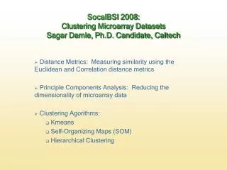
SocalBSI 2008:Clustering Microarray DatasetsSagar Damle, Ph.D. Candidate, Caltech Distance Metrics: Measuring similarity using the Euclidean and Correlation distance metrics Principle Components Analysis: Reducing the dimensionality of microarray data Clustering Agorithms: Kmeans Self-Organizing Maps (SOM) Hierarchical Clustering
MATRIXgenes,conditions = Expression datasetthe first genevector = (x11, x12, x13, x14… x1n)the leftmost condition vector = (x11, x21, x31 … xm1) Columns (conditions [timepoints, or tissues]) x11 , x12 , x13 , … x1n x21 x31 , … Xm1 … xmn Rows (genes)
Similarity measures • Clustering identifies group of genes with “similar” expression profiles • How is similarity measured? • Euclidian distance • Correlation coefficient • Others: Manhattan, Chebychev, Euclidean Squared
In an experiment with 10 conditions, the gene expression profiles for two genes X, and Y would have this form X = (x1, x2, x3, …, x10) Y = (y1, y2, y3, …, y10)
d(Ga, Gb) = sqrt( (x1-y1)2 + (x2 -y2)2 ) Similarity measure - Euclidian distance Gb: (x1, x2) Ga: (y1, y2) In general: if there are M experiments: X = (x1, x2, x3, …, xm) Y = (y1, y2, y3, …, ym)
Similarity measure – Pearson Correlation Coefficient X = (x1, x2, x3, …, xm), Y = (y1, y2, y3, …, ym) • D = 1 - r • r = [Z(X)*Z(Y)] (dot product of the z-scores of vectors X and Y) • r = |Z(X)| |Z(Y)| cos(T) • When two unit vectors are completely correlated, r=1 and D=0 • When two unit vectors are non correlated, r=0 and D = 1 • Dot product review: http://mathworld.wolfram.com/DotProduct.html
Euclidian vs Pearson Correlation • Euclidian distance – takes into account the magnitude of the expression • Correlation distance - insensitive to the amplitude of expression, takes into account the trends of the change. • Common trends are considered biologically relevant, the magnitude is considered less important Gene Y Gene X
What euclidean distance sees What correlation distance sees
Principle Components Analysis (PCA) • A method for projecting microarray data onto a reduced (2 or 3 dimensional) easily visualized space Definition: Principle Components - A set of variables that define a projection that encapsulates the maximum amount of variation in a dataset and is orthogonal (and therefore uncorrelated) to the previous principle component of the same dataset. • Example Dataset: Thousands of genes probed in 10 conditions. • The expression profile of each gene is presented by the vector of its expression levels: X = (X1, X2, X3, X4, X5) • Imagine each gene X as a point in a 5-dimentional space. • Each direction/axis corresponds to a specific condition • Genes with similar profiles are close to each other in this space • PCA- Project this dataset to 2 dimensions, preserving as much information as possible
PCA transformation of a microarray dataset Visual estimation of the number of clusters in the data
1-page tutorial on singular value decomposition (PCA) http://web.mit.edu/be.400/www/SVD/Singular_Value_Decomposition.htm
Cluster analysis Function • Places genes with similar expression patterns in groups. • Sometimes genes of unknown function will be grouped with genes of known function. • The functions that are known allow the investigator to hypothesize regarding the functions of genes not yet characterized. • Examples: • Identify genes important in cell cycle regulation • Identify genes that participate in a biosynthetic pathway • Identify genes involved in a drug response • Identify genes involved in a disease response
Clustering yeast cell cycle dataset VS gene tree ordering
How to choose the number of clusters needed to informatively partition the data Trial and error: Try clustering with a different number of clusters, and compare your results • Criteria for comparison: Homogeneity vs Separation • Use PCA (Principle Component Analysis) to visually determine how well the algorithm grouped genes • Calculate the mean distance between all genes within a cluster (it should be small) and compare that to the distance between clusters (which should be large)
Mathematical evaluation of clustering solution Merits of a ‘good’ clustering solution: • Homogeneity: • Genes inside a cluster are highly similar to each other. • Average similarity between a gene and the center (average profile) of its cluster. • Separation: • Genes from different clusters have low similarity to each other. • Weighted average similarity between centers of clusters. • These are conflicting features: increasing the number of clusters tends to improve with-in cluster Homogeneity on the expense of between-cluster Separation
Performance on Yeast Cell Cycle Data CAST* “True” CLICK GeneCluster Separation K-means Homogeneity 698 genes, 72 conditions (Spellman et al. 1998). Each algorithm was run by its authors in a “blind” test. *Ben-Dor, Shamir, Yakhini 1999
Clustering Algorithms • K–means • SOMs • Hierarchical clustering
K-MEANS • The user sets the number of clusters- k • Initialization: each gene is randomly assigned to one of the k clusters • Average expression vector is calculated for each cluster (cluster’s profile) • Iterate over the genes: • For each gene- compute its similarity to the cluster profiles. • Move the gene to the cluster it is most similar to. • Recalculated cluster profiles. • Score current partition: sum of distances between genes and the profile of the cluster they are assigned to (homogeneity of the solution). • Stop criteria: further shuffling of genes results in minor improvement in the clustering score
Mean profile Standard deviation in each condition K-MEANS example: 4 clusters (too many?)
Evaluating Kmeans Cluster 1 Cluster 3 Mis-classified Cluster 4 Cluster 2
SOMs (Self-Organizing Maps)less clustering and more data organizing • User sets the number of clusters in a form of a rectangular grid (e.g., 3x2) – ‘map nodes’ • Imagine genes as points in (M-dimensional) space • Initialization: map nodes are randomly placed in the data space
Genes – data points Clusters – map nodes
SOM - Scheme • Randomly choose a data point (gene). • Find its closest map node • Move this map node towards the data point • Move the neighbor map nodes towards this point, but to lesser extent (thinner arrows show weaker shift) • Iterate over data points
Each successive gene profile (black dot) has less of an influence on the displacement of the nodes. • Iterate through all profiles several times (10-100) • When positions of the cluster nodes have stabilized, assign each gene to its closest map node (cluster)
{1,2,3,4,5} {1,2,3} {4,5} {1,2} g1 g2 g3 g4 g5 Hierarchical Clustering • Goal#1: Organize the genes in a structure of a hierarchical tree • 1) Initial step: each gene is regarded as a cluster with one item • 2) Find the 2 most similar clusters and merge them into a common node (red dot) • 3) Merge successive nodes until all genes are contained in a single cluster • Goal#2: Collapse branches to group genes into distinct clusters
Which genes to cluster? • Apply filtering prior to clustering – focus the analysis on the ‘responding genes’ • The application of controlled statistical tests to identify ‘responding genes’ usually ends up with too few genes that do not allow for a global characterization of the response. • Variance: filter out genes that do not vary greatly among the conditions of the experiment. • Non-varying genes skew clustering results, especially when using a correlation coefficient • Fold change: choose genes that change by at least M-fold in at least L conditions.
Clustering – Tools • Cluster (Eisen) – hierarchical clustering • http://rana.lbl.gov/EisenSoftware.htm • GeneCluster (Tamayo) – SOM • http://bioinfo.cnio.es/wwwsomtree/ • TIGR MeV – K-Means, SOM, hierarchical, QTC, CAST • http://www.tm4.org/mev.html • Expander – CLICK, SOM, K-means, hierarchical • http://www.cs.tau.ac.il/~rshamir/expander/expander.html • Many others (e.g. GeneSpring) • http://www.agilent.com/chem/genespring
Analysis Strategy • Transform Dataset Using PCA • Cluster • Parameters to test: • Distance Metric • Number of clusters • Separation & Homogeneity • Assign biological meaning to clusters
Original presentation created by Rani Elkon and posted at: http://www.tau.ac.il/lifesci/bioinfo/teaching/2002-2003/DNA_microarray_winter_2003.html