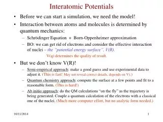
Interatomic Potentials
Before conducting simulations, a model for the interaction between atoms and molecules is crucial, which is determined by quantum mechanics, such as the Schrödinger Equation and Born-Oppenheimer approximation. Different approaches like semi-empirical, quantum chemistry, and ab initio methods are used to determine the potential energy surface V(R) for accurate results. The non-relativistic Hamiltonian in atomic units necessitates high accuracy for room temperature simulations. Different potential models, including atom-atom potentials and atomic systems, consider factors like molecular geometry, short-range, electrostatic, and dispersion effects. The Lennard-Jones potential and its application in molecular dynamics are discussed, along with the Morse potential for bonded atoms.
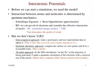

Interatomic Potentials
E N D
Presentation Transcript
Interatomic Potentials • Before we can start a simulation, we need the model! • Interaction between atoms and molecules is determined by quantum mechanics: • Schrödinger Equation + Born-Oppenheimer approximation • BO: we can get rid of electrons and consider the effective interaction of nuclei – the “potential energy surface”, V(R). V(q) determines the quality of result. • But we don’t know V(R)! • Semi-empirical approach: make a good guess and use experimental data to adjust it. (This is fast! May not reveal correct details, depends on V).) • Quantum chemistry approach: compute the surface at a few points and fit to a reasonable form. (This is hard!) • Ab initio approach: do the QM calculations “on the fly” as the trajectory is being generated. Couple a quantum calculation of the electrons with a classical one of the nuclei. (Much more computer effort, but no analytic form needed.)
The electronic-structure problem The non-relativistic Hamiltonian for a collection of ions and electrons: “Atomic units”: Energy in Hartrees=27.2eV=316,000K Lengths in Bohr radii= 0.529 A = 5.29 x10⁻⁹cm • Accuracy needed to address questions at room temp.: 100 K=0.3 mHa=0.01eV. • MANY DECIMAL PLACES! Solving this is difficult!
Born-Oppenheimer (1927) Approximation • Make use of the fact that nuclei are so much heavier than electrons. • Worse case: proton mass= 1836 electron mass. Electrons move much faster! • Factor total wavefunction into ionic and electronic parts. (adiabatic approx) electronic and nuclear parts • Does not mean that the ions are classical! (but MD assumes it) • Eliminate the electrons and replace by an effective potential.
Semi-empirical potentials • What data? • Molecular bond lengths, binding energies • Atom-atom scattering in gas phase • Virial coefficients, transport in gas phase • Low temperature properties of the solid, cohesive energy, lattice constant, elastic moduli, vibrational frequencies, defect energies. • Melting temperature, critical point, triple point, surface tension,…. • GIGO, i.e. “garbage in, garbage out”! • Interpolation versus extrapolation: “transferability” • Are results predictive? • How much theory to use, and how much experimental data? • Assume a functional form, e.g., a 2-body or 3-body. • Find some data from experiment. • Use theory+simulation to determine parameters.
Atom-Atom potentials • Total potential is the sum of atom-atom pair potentials • Assumes molecule is rigid, in non-degenerate ground state, interaction is weak so the internal structure is weakly affected by the environment. • Geometry (steric effect) is important. • Short-range effects-repulsion caused by cores: exp(-r/c) • Perturbation theory as rij >> core radius • Electrostatic effects: do a multipole expansion (if charged or have dipoles) • Induction effects (by a charge on a neutral atom) • Dispersion effects: dipole-induced-dipole (C6/r6)
Atomic systems • Neutral rare gas atoms are the simplest atoms to find a potential for: little attractive spheres. • Repulsion at short distances because of overlap of atomic cores. • Attraction at long distance die to the dipole-induced-dipole force. Dispersion interaction is c6r-6 + c8 r-8 + …. • He-He interaction is the most accurate. Use all available low density data (virial coefficients, quantum chemistry calculations, transport coefficients, ….) Good to better than 0.1K (work of Aziz over last 20 years). But that system needs quantum simulations. Three-body (and many-body) interactions are small but not zero. • Good potentials are also available for other rare gas atoms. • H2 is almost like rare gas from angular degree of freedom averages out due to quantum effects. But has a much larger polarizability.
Lennard-Jones (2-body) potential ~ minimum = wall of potential • Good model for non-bonded rare gas atoms • Standard model for MD! • Why these exponents? 6 and 12? • There is only 1 LJ system! • Reduced units: • Energy in : T*=kBT/ • Lengths in : x=r/ • Time is mass units, pressure, density,.. • See references on FS pgs. 51-54
! Loop over all pairs of atoms. do i=2,natoms do j=1,i-1 !Compute distance between i and j. r2 = 0 do k=1,ndim dx(k) = r(k,i) - r(k,j) !Periodic boundary conditions. if(dx(k).gt. ell2(k)) dx(k) = dx(k)-ell(k) if(dx(k).lt.-ell2(k)) dx(k) = dx(k)+ell(k) r2 = r2 + dx(k)*dx(k) enddo !Only compute for pairs inside radial cutoff. if(r2.lt.rcut2) then r2i=sigma2/r2 r6i=r2i*r2i*r2i !Shifted Lennard-Jones potential. pot = pot+eps4*r6i*(r6i-1)- potcut !Radial force. rforce = eps24*r6i*r2i*(2*r6i-1) do k = 1 , ndim force(k,i)=force(k,i) + rforce*dx(k) force(k,j)=force(k,j) - rforce*dx(k) enddo endif enddo enddo LJ Force Computation
Phase diagram of Lennard-Jones A. Bizjak, T.Urbi and V. VlachyActa Chim. Slov. 2009, 56, 166–171
Morse potential • Like Lennard-Jones but for bonded atoms • Repulsion is more realistic - but attraction less so. • Minimum at r0 , approximately the neighbor position • Minimum energy is • An extra parameter “a” that can be used to fit a third property: lattice constant (r0 ), bulk modulus (B) and cohesive energy.
Various Other Empirical Potentials Hard sphere - simplest, first, no integration error. b) Hard sphere, square well c) Coulomb (long-ranged) for plasmas d) 1/r12 potential (short-ranged)
Fit for a Born potential • Attractive charge-charge interaction • Repulsive interaction determined by atom core. EXAMPLE: NaCl • Obviously Zi = 1 on simple cubic structure/alternating charges • Use cohesive energy and lattice constant (at T=0) to determine A and n n=8.87 A=1500eV|8.87 • Now we need a check, say, the “bulk modulus”. • We get 4.35 x 10¹¹ dy/cm2Experiment = 2.52 x 10¹¹ dy/cm2 • You get what you fit for!
Arbitrary Pair Potential • For anything more complicated than a LJ 6-12 potential you can use a table-driven method. • In start up of MD, compute or read in a table of potential values. e.g. V(ri), dV/dr on a table. • During computation, map interatomic distance to a grid and compute grid index and difference • Do table look-up and compute (cubic) polynomial. • Complexity is memory fetch+a few flops/distance • Advantage: Code is completely general-can handle any potential at the same cost. • Disadvantage: some cost for memory fetch. (cache misses)
Failure of pair potentials • Ec=cohesive energy and Ev=vacancy formation energy • Tm=melting temperature • C12 and C44 are shear elastic constants. • A “Cauchy” relation makes them equal in a cubic lattice for any pair potential. • Problem in metals: electrons are not localized! After Ercolessi, 1997
Metallic potentials • Have a inner core + valence electrons • Valence electrons are delocalized. • Hence pair potentials do not work very well. Strength of bonds decreases as density increases because of Pauli principle. • EXAMPLE: at a surface LJ potential predicts expansion but metals contract. • Embedded Atom Model (EAM) or glue models work better. Daw and Baskes, PRB 29, 6443 (1984). • Three functions to optimize! • Good for spherically symmetric atoms: Cu, Pb • Not for metals with covalent bonds or metals (Al) with large changes in charge density under shear.
rk ri i rj Silicon potential • Solid silicon can not be described with a pair potential. • Has open structure, with coordination 4! • Tetrahedral bonding structure caused by the partially filled p-shell. • Very stiff potential, short-ranged caused by localized electrons: • Stillinger-Weber (Phys. Rev. B 31, 5262, 1985) potential fit from: Lattice constant,cohesive energy, melting point, structure of liquid Si for r<a • Minimum at 109o
Hydrocarbon potential • Empirical potentials to describe intra- molecular and inter-molecular forces • AMBER potential is: • Two-body Lennard-Jones+ charge interaction (non-bonded) • Bonding potential: kr(ri-rj)2 • Bond angle potential ka(- 0)2 • Dihedral angle: vn[ 1 - cos(n)] • All parameters taken from experiment. • Rules to decide when to use which parameter. • Several “force fields” available • (open source/commercial).
Water potentials Mahoney & Jorgensen • Older potentials: BNS,MCY,ST2 • New ones: TIP3P,SPC,TIP4P • TIP5P • Rigid molecule with 5 sites • Oxygen in center that interacts with other oxygens using LJ 6-12 • 4 charges (e = 0.24) around it so it has a dipole moment • Compare with phase diagram (melting and freezing), pair correlations, dielectric constant
Problems with potentials • Potential is highly dimensional function. Arises from QM so it is not a simple function. • Procedure: fit data relevant to the system you are going to simulate: similar densities and local environment. • Use other experiments to test potential. • Do quantum chemical (SCF or DFT) calculations of clusters. Be aware that these may not be accurate enough. • Noempirical potentials work very well in an inhomogenous environment. • This is the main problem with atom-scale simulations--they really are only suggestive since the potential may not be correct. Universality helps (i.e., sometimes the potential does not matter that much)
Which approach to use? • Type of systems: metallic, covalent, ionic, van der Waals • Desired accuracy: quantitative or qualitative • Transferability: many different environments • Efficiency: system size and computer resources • (10 atoms or 108atoms. 100fs or 10 ms) Total error is the combination of: • statistical error(the number of time steps) • systematic error (the potential)