The arithmetic mean is the "standard" average, often simply called the "mean "

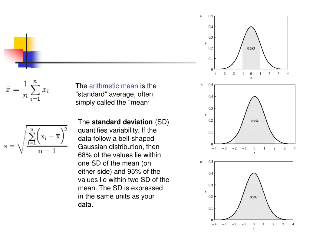
1. The arithmetic mean is the "standard" average, often simply called the "mean" The standard deviation (SD) quantifies variability. If the data follow a bell-shaped Gaussian distribution, then 68% of the values lie within one SD of the mean (on either side) and 95% of the values lie within two SD of the mean. The SD is expressed in the same units as your data.

2. Errors separate into two broad categories: those originating from the analyst and those originating with the method. The former is an error that is due to poor execution, the latter an error due to an inherent problem with the method. Method validation is designed to minimize and characterize method error. Minimization of analyst error involves education and training. A second way to categorize errors is by whether they are systematic. Systematic errors are predictable and impart a bias to reported results. These errors are usually easy to detect by using blanks, calibration checks, and controls. In a validated method, bias is minimal and well characterized. Random errors are equally positive and negative and are generally small.

4. CALIBRATION OF EQUIPMENT The accuracy and precision of analytical devices must be known and monitored. Devices requiring calibration include refrigerators, balances, pipets, syringes, pH meters, microscopes, and so on. In short, if the equipment provides a measurement that is related to generating data, it must be calibrated. Suppose an Eppendorf pipet arrives at a lab. The analyst immediately validates this performance by repeatedly pipetting what the device records as aliquots into dried, tared containers on a calibrated analytical balance. By recording the water temperature and using a chart that relates density to temperature, the analyst converts the weight of water, in milligrams, to a volume delivered by the pipet.

5. CALIBRATION OF INSTRUMENTS: CONCENTRATION AND RESPONSE This type of calibration, typically for instruments like spectrometers, requires the use of linear regression. earlier in the chapter. A good regression line is required for a valid calibration. A calibration curve has a lifetime that is linked to the stability of the instrument and the calibration standards. Another aspect of curve validation is the use of calibration checks. The ideal calibration check (CC) is obtained from a traceable standard that is independent of the solutions used to prepare the calibration standards. This is the only method that facilitates the detection of a problem in the stock solution. Finally, blanks must be analyzed regularly to ensure that equipment and instrumentation have not been contaminated Thus, four factors contribute to the validation of a calibration curve: correlation coefficient (R2), the absence of a response to a blank the time elapsed since the initial calibration or update, and performance on an independent calibration-check sample.

6. The goodness of fit of the line is measured by the correlation coefficient or more frequently as its squared value R2, and is a measure of linearity of the points. If the line is perfectly correlated and has a positive slope whereas describes a perfectly correlated line with a negative slope. If there is no correlation, It is important to remember that r is but one measure of the goodness of a calibration curve, and all curves should be inspected visually as a second level of control.

7. PREDICTIVE MODELING AND CALIBRATION Involves multivariate statistics (the application of statistics to data sets with more than one variable) Regression lines take the familiar form (y = mx + b ) where m is the slope and b is the y-intercept, or simply intercept. The variable y is called the dependent variable, since its value is dictated by x, the independent variable. All linear calibration curves share certain generic features. The range in which the relationship between concentration and response is linear is called the linear range and is typically described by “orders of magnitude.” A calibration curve that is linear from 1 ppb to 1 ppm, a factor of 1000, has a linear dynamic range (LDR) of three orders of magnitude. At higher concentrations, most detectors become saturated and the response flattens out; the calibration curve is not valid in this range of higher concentrations, and samples with concentrations above the last linear point on the curve must be diluted before quantitation. The concentration corresponding to the lowest concentration in the linear range is called the limit of quantitation (LOQ). Instruments may detect a response below this concentration, but it is not predictable and the line cannot be extrapolated to concentrations smaller than the LOQ. The concentration at which no significant response can be detected is the limit of detection, or LOD.

8. The line generated by a least-squares regression results from fitting empirical data to a line that has the minimum total deviation from all of the points. The method is called least squares because distances from the line are squared to prevent points that are displaced above the line (signified by a plus sign, ) from canceling those displaced below the line (signified by a minus sign, ). Most linear regression implementations have an option to “force the line through the origin,” which means forcing the intercept of the line through the point (0,0). This might seem reasonable, since a sample with no detectable cocaine should produce no response in a detector, but must be used with care.

9. Forcing the plot through (0,0)is not always recommended, since most curves are run well above the instrumental limit of detection (LOD). Arbitrarily adding a point (0,0) can skew the curve because the instrument’s response near the LOD is not predictable and is rarely linear, as show below. As illustrated forcing a curve through the origin can, under some circumstances, bias results.

10. CALIBRATION OF INSTRUMENTS: CONCENTRATION AND RESPONSE • External Standard: This type of curve is familiar to students as a simple concentration- versus-response plot fit to a linear equation. Standards are prepared in a generic solvent, such as methanol for organics or 1% acid for elemental analyses. Such curves are easy to generate, use, and maintain. For example, if an analysis is to be performed on cocaine, some sample preparation and cleanup is done and the matrix removed or diluted away. In such cases, most interference from the sample matrix is inconsequential, and an external standard is appropriate. External standard curves are also used when internal standard calibration is not feasible, as in the case of atomic absorption spectrometry. • Internal Standard: External standard calibrations can be compromised by complex or variable matrices. In toxicology, blood is one of the more difficult matrices to work with, because it is a thick, viscous liquid containing large and small molecular components, proteins, fats, and many materials subject to degradation. A calibration curve generated in an organic solvent is dissimilar from that generated in the sample matrix, a phenomenon called matrix mismatch. Internal standards provide a reference to which concentrations and responses can be ratioed. The use of an internal standard requires that the instrument system respond to more than one analyte at a time. Furthermore, the internal standard must be carefully selected to mimic the chemical behavior or the analytes.

11. Example: Calibration standards are prepared from a certified stock solution of cocaine in methanol, which is diluted to make five calibration standards. The laboratory prepares a calibration check in a diluted blood solution using certified standards, and the concentration of the resulting mixture is 125.0 ppb cocaine. When this solution is analyzed with the external- standard curve, the calculated concentration is found to be about half of the known true value. The reason for the discrepancy is related to the matrix, in which unknown interactions mask nearly half of the cocaine present.

13. Now consider an internal-standard approach An internalstandard of xylocaine is chosen because it is chemically similar to cocaine, but unlikely to be found in typical samples. To prepare the calibration curve, cocaine standards are prepared as before, but 75.0 ppb of xylocaine is included in all calibration solutions.