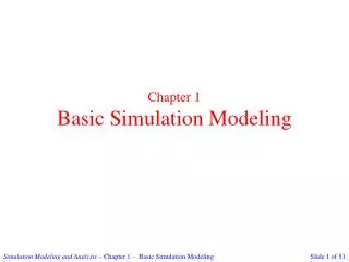
Modeling & Simulation
Modeling & Simulation. Experimental Frame. Simulator. Source System. Modeling Relation. Simulation Relation. Model. System Models and Simulation. Framework for Modeling and Simulation The framework defines the entities and their Relationships that are central to the M&S enterprise.

Modeling & Simulation
E N D
Presentation Transcript
Experimental Frame Simulator Source System Modeling Relation Simulation Relation Model System Models and Simulation • Framework for Modeling and SimulationThe framework defines the entities and their Relationships that are central to the M&S enterprise Figure 1 Basic Entities in M&S Framework and their Relationships
1-The source system : is the real or virtual environment that we interested in modeling (it is viewed as a source of observable data). 2-Experimental Frame : is a specification of the conditions under which the system is observed or experimented with. 3- Simulation Model : It is a set of instructions, rules, equations, or constrains for generating I/O behavior of the system. 4- Simulator: any computation system that Capable of executing the model to generate its behavior (Processor, Human Mind, or an algorithm).
Definitions: • System’s state:is the collection of variables (state variables) necessary to describe a system at a particular time, relative to the objectives of a study. • Systems Types: We categorize systems to be of two types, discrete and continuous. • A discrete system :is one for which the state variables change instantaneously at separated points in time. • A continuous system : is one for which the state variables change continuously with respect to time.
Static vs. Dynamic Simulation Models: A static simulation model is a representation of a system at a particular time, a dynamic simulation model represents a system as it evolves over time, such as a conveyor system in a factory. • Continuous vs. Discrete Simulation Models: a discrete model is not always used to model a discrete system and vice versa. To use a discrete or a continuous model for a particular system depends on the specific objectives of the study.
Deterministic vs. Stochastic Simulation Models: If a simulation model does not contain any probabilistic (i.e., random) components, it is called deterministic; Stochastic simulation models:Having at least some random input components produce output that is itself random.
Discrete-Event Simulation • Discrete-event simulation concerns the modeling of a system as it evolves over time by a representation in which the state variables change instantaneously at separate points in time. These points in time are the ones at which an event occurs. • Event is defined as an instantaneous occurrence that may change the state of the system.
Example 1 : Consider a service facility with a single server • State variables: that may be used to simulate this system are: - Status of the server (idle or busy) - Number of customers waiting in a queue - Time of arrival for each customer. • Events for this system: - The arrival of a customer - The completion of service for a customer,
Simulation of A Single-Server Queuing System • Problem Statement Consider a single-server queuing system :
D2 • ti: times of arrival of the ith customer (t0=0) • Ai= ti -ti-1 the interarrival time between (i-1)st and ith arrivals of customers. • Si: service time for the ith customer • Di : Delay in queue for the ith customer • Ci = ti + Di +Si • ei: time of occurrence of ith event.
the interarrival times A1, A2, … are independent, identically distributed (IID) random variables. • the service times S1, S2, … of the successive customers are IID random variables that are independent of the interarrival times. • We wish to simulate this system until a fixed number (n) of customers have completed their delays in queue.
Measures of performance To measure the performance of this system, we will look at estimates of three quantities: 1-The expected average delay in queue of the n customers completing their delays during the simulation; we denote this quantity by d (n). • From a single run of the simulation resulting in customer delays D1, D2, ….., Dn, an obvious estimator of d(n) is • Which is just the average of the n Di’s
2- The expected average number of customers in the queue, denoted by q(n ) • Let Q (t): denote the number of customers in queue at time t, for any real number t ≥ 0 • T (n) : be the total time required to observe our n delays in queue of length i. Ť(n) = T0 + T1 + T2 + ….
(1.1) • : is the observed proportion of the time during the simulation that there were i customers in the queue. • = Ti / T(n), so that we can rewrite Eq. (1.1) above as : (1.2)
3- The expected utilization of the server • Which isthe expected proportion of time during the simulation that the server is busy (i.e., not idle), denote it by u (n). • our estimate of u(n) is û(n) = the observed proportion of time during the simulation that the server is busy.
Components and Organization of a Discrete-Event Simulation Model In particular, the following components will be found in most discrete-event simulation models using the next-event time-advance approach: • System state: The collection of state variables necessary to describe the system at a particular time. • Simulation clock: A variable giving the current value of simulated time. • Event list: A list containing the next time when each type of event will occur. • Statistical counters: Variables used for storing statistical information about system performance. • Initialization routine: A subprogram to initialize the simulation model at time zero.
Timing routine: A subprogram that determines the next event from the event list and then advances the simulation clock to the time when that event is to occur. • Event routine: A subprogram that updates the system state when a particular type of event occurs. • Report generator: A subprogram that computes estimates (from the statistical counters) of the desired measures of performance and produces a report when the simulation ends. • Main program: A subprogram that invokes the timing routine to determine the next event and then transfers state control to the corresponding event routine to update the system state appropriately. The main program may also check for termination and invoke the report generator when simulation is over