Design Issues for Paging Systems
Design Issues for Paging Systems. The Working Set Model

Design Issues for Paging Systems
E N D
Presentation Transcript
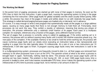
Design Issues for Paging Systems The Working Set Model In the purest form of paging, processes are started up with none of their pages in memory. As soon as the CPU tries to fetch the first instruction, it gets a page fault, causing the operating system to bring in the page containing the first instruction. Other page faults for global variables and the stack usually follow quickly. After a while, the process has most of the pages it needs and settles down to run with relatively few page faults. This strategy is called demand paging because pages are loaded only on demand, not in advance. Of course, it is easy enough to write a test program that systematically reads all the pages in a large address space, causing so many page faults that there is not enough memory to hold them all. Fortunately, most processes do not work this way. They exhibit a locality of reference, meaning that during any phase of execution, the process references only a relatively small fraction of its pages. Each pass of a multipass compiler, for example, references only a fraction of the pages, and a different fraction at that. The set of pages that a process is currently using is called its working set. If the entire working set is in memory, the process will run without causing many faults until it moves into another execution phase (e.g., the next pass of the compiler). If the available memory is too small to hold the entire working set, the process will cause numerous page faults and run slowly since executing an instruction takes a few nanoseconds and reading in a page from the disk typically takes 10 milliseconds. At a rate of one or two instructions per 10 milliseconds, it will take ages to finish. A program causing page faults every few instructions is said to be thrashing. In a multiprogramming system, processes are frequently moved to disk (i.e., all their pages are removed from memory) to let other processes have a turn at the CPU. The question arises of what to do when a process is brought back in again. Technically, nothing need be done. The process will just cause page faults until its working set has been loaded. The problem is that having 20, 100, or even 1000 page faults every time a process is loaded is slow, and it also wastes considerable CPU time, since it takes the operating system a few milliseconds of CPU time to process a page fault, not to mention a fair amount of disk I/O.
Therefore, many paging systems try to keep track of each process' working set and make sure that it is in memory before letting the process run. This approach is called the working set model. It is designed to greatly reduce the page fault rate. Loading the pages before letting processes run is also called prepaging. Note that the working set changes over time. It has long been known that most programs do not reference their address space uniformly. Instead the references tend to cluster on a small number of pages. A memory reference may fetch an instruction, it may fetch data, or it may store data. At any instant of time, t, there exists a set consisting of all the pages used by the k most recent memory references. This set, w(k, t), is the working set. Because a larger value of k means looking further into the past, the number of pages counted as part of the working set cannot decrease as k is made larger. So w(k, t) is a monotonically nondecreasing function of k. The limit of w(k, t) as k becomes large is finite because a program cannot reference more pages than its address space contains, and few programs will use every single page. Figure 1 depicts the size of the working set as a function of k. Figure 1. The working set is the set of pages used by the k most recent memory references. The function w(k, t) is the size of the working set at time t. The fact that most programs randomly access a small number of pages, but that this set changes slowly in time explains the initial rapid rise of the curve and then the slow rise for large k. For example, a program that is executing a loop occupying two pages using data on four pages, may reference all six pages every 1000 instructions, but the most recent reference to some other page may be a million instructions earlier, during the initialization phase. Due to this asymptotic behavior, the contents of the working set is not sensitive to the value of k chosen. To put it differently, there exists a wide range of k values for which the working set is unchanged.
Local versus Global Allocation Policies In the preceding sections we have discussed several algorithms for choosing a page to replace when a fault occurs. A major issue associated with this choice (which we have carefully swept under the rug until now) is how memory should be allocated among the competing runnable processes. Take a look at Fig. 2(a). In this figure, three processes, A, B, and C, make up the set of runnable processes. Suppose A gets a page fault. Should the page replacement algorithm try to find the least recently used page considering only the six pages currently allocated to A, or should it consider all the pages in memory? If it looks only at A's pages, the page with the lowest age value is A5, so we get the situation of Fig 2(b) Figure 2. Local versus global page replacement. (a) Original configuration. (b) Local page replacement. (c) Global page replacement. On the other hand, if the page with the lowest age value is removed without regard to whose page it is, page B3 will be chosen and we will get the situation of Fig. 2(c). The algorithm of Fig. 2(b) is said to be a local page replacement algorithm, whereas that of Fig. 2(c) is said to be a global algorithm. Local algorithms effectively correspond to allocating every process a fixed fraction of the memory. Global algorithms dynamically allocate page frames among the runnable processes. Thus the number of page frames assigned to each process varies in time.
In general, global algorithms work better, especially when the working set size can vary over the lifetime of a process. If a local algorithm is used and the working set grows, thrashing will result, even if there are plenty of free page frames. If the working set shrinks, local algorithms waste memory. If a global algorithm is used, the system must continually decide how many page frames to assign to each process. One way is to monitor the working set size as indicated by the aging bits, but this approach does not necessarily prevent thrashing. Another approach is to have an algorithm for allocating page frames to processes. One way is to periodically determine the number of running processes and allocate each process an equal share. Thus with 12,416 available (i.e., nonoperating system) page frames and 10 processes, each process gets 1241 frames. The remaining 6 go into a pool to be used when page faults occur. Although this method seems fair, it makes little sense to give equal shares of the memory to a 10-KB process and a 300-KB process. Instead, pages can be allocated in proportion to each process' total size, with a 300-KB process getting 30 times the allotment of a 10-KB process. It is probably wise to give each process some minimum number, so it can run, no matter how small it is. On some machines, for example, a single two-operand instruction may need as many as six pages because the instruction itself, the source operand, and the destination operand may all straddle page boundaries. With an allocation of only five pages, programs containing such instructions cannot execute at all. If a global algorithm is used, it may be possible to start each process up with some number of pages proportional to the process' size, but the allocation has to be updated dynamically as the processes run. One way to manage the allocation is to use the PFF (Page Fault Frequency) algorithm. It tells when to increase or decrease a process' page allocation but says nothing about which page to replace on a fault. It just controls the size of the allocation set. For a large class of page replacement algorithms, including LRU, it is known that the fault rate decreases as more pages are assigned, as we discussed above. This is the assumption behind PFF. This property is illustrated in Figure 3.
Figure 3. Page fault rate as a function of the number of page frames assigned. Measuring the page fault rate is straightforward: just count the number of faults per second, possibly taking a running mean over past seconds as well. One easy way to do this is to add the present second's value to the current running mean and divide by two. The dashed line marked A corresponds to a page fault rate that is unacceptably high, so the faulting process is given more page frames to reduce the fault rate. The dashed line marked B corresponds to a page fault rate so low that it can be concluded that the process has too much memory. In this case, page frames may be taken away from it. Thus, PFF tries to keep the paging rate for each process within acceptable bounds. If it discovers that there are so many processes in memory that it is not possible to keep all of them below A, then some process is removed from memory, and its page frames are divided up among the remaining processes or put into a pool of available pages that can be used on subsequent page faults. The decision to remove a process from memory is a form of load control. It shows that even with paging, swapping is still needed, only now swapping is used to reduce potential demand for memory, rather than to reclaim blocks of it for immediate use. Swapping processes out to relieve the load on memory is reminiscent of two-level scheduling, in which some processes are put on disk and a short-term scheduler is used to schedule the remaining processes. Clearly, the two ideas can be combined, with just enough processes swapped out to make the page-fault rate acceptable.
Page Size The page size is often a parameter that can be chosen by the operating system. Even if the hardware has been designed with, for example, 512-byte pages, the operating system can easily regard pages 0 and 1, 2 and 3, 4 and 5, and so on, as 1-KB pages by always allocating two consecutive 512-byte page frames for them. Determining the best page size requires balancing several competing factors. As a result, there is no overall optimum. To start with, there are two factors that argue for a small page size. A randomly chosen text, data, or stack segment will not fill an integral number of pages. On the average, half of the final page will be empty. The extra space in that page is wasted. This wastage is called internal fragmentation. With n segments in memory and a page size of p bytes, np/2 bytes will be wasted on internal fragmentation. This argues for a small page size. Another argument for a small page size becomes apparent if we think about a program consisting of eight sequential phases of 4 KB each. With a 32-KB page size, the program must be allocated 32 KB all the time. With a 16-KB page size, it needs only 16 KB. With a page size of 4 KB or smaller, it requires only 4 KB at any instant. In general, a large page size will cause more unused program to be in memory than a small page size. On the other hand, small pages mean that programs will need many pages, hence a large page table. A 32-KB program needs only four 8-KB pages, but 64 of 512-byte pages. Transfers to and from the disk are generally a page at a time, with most of the time being for the seek and rotational delay, so that transferring a small page takes almost as much time as transferring a large page. It might take 64 x 10 msec to load 64 512-byte pages, but only 4 x 10.1 msec to load four 8-KB pages. On some machines, the page table must be loaded into hardware registers every time the CPU switches from one process to another. On these machines having a small page size means that the time required to load the page registers gets longer as the page size gets smaller. Furthermore, the space occupied by the page table increases as the page size decreases. This last point can be analyzed mathematically. Let the average process size be s bytes and the page size be p bytes. Furthermore, assume that each page entry requires e bytes. The approximate number of pages needed per process is then s/p, occupying se/p bytes of page table space. The wasted memory in the last page of the process due to internal fragmentation is p/2. Thus, the total overhead due to the page table and the internal fragmentation loss is given by the sum of these two terms: overhead = se/p + p/2 The first term (page table size) is large when the page size is small. The second term (internal fragmentation) is large when the page size is large. The optimum must lie somewhere in between. By taking the first derivative with respect to p and equating it to zero, we get the equation From this equation we can derive a formula that gives the optimum page size (considering only memory wasted in fragmentation and page table size). The result is:
Segmentation An important aspect of memory management that became unavoidable with paging is the separation of the user's view of memory and the actual physical memory. As we have already seen, the user's view of memory is not the same as the actual physical memory. The user's view is mapped onto physical memory. This mapping allows differentiation between logical memory and physical memory. Basic Method Do users think of memory as a linear array of bytes, some containing instructions and others containing data? Most people would say no. Rather, users prefer to view memory as a collection of variable-sized segments, with no necessary ordering among segments (Figure 4). Consider how you think of a program when you are writing it. You think of it as a main program with a set of methods, procedures, or functions. It may also include various data structures: objects, arrays, stacks, variables, and so on. Each of these modules or data elements is referred to by name. You talk about “the stack," "the math library”, “the main program”, without caring what addresses in memory these elements occupy. Figure 4. User’s view of a program
You are not concerned with whether the stack is stored before or after the Sqrt() function. Each of these segments is of variable length; the length is intrinsically defined by the purpose of the segment in the program. Elements within a segment are identified by their offset from the beginning of the segment: the first statement of the program, the seventh stack frame entry in the stack, the fifth instruction of the Sqrt () , and so on. • Segmentation is a memory-management scheme that supports this user view of memory. A logical address space is a collection of segments. Each segment has a name and a length. The addresses specify both the segment name and the offset within the segment. The user therefore specifies each address by two quantities: a segment name and an offset. (Contrast this scheme with the paging scheme, in which the user specifies only a single address, which is partitioned by the hardware into a page number and an offset, all invisible to the programmer.) • For simplicity of implementation, segments are numbered and are referred to by a segment number, rather than by a segment name. Thus, a logical address consists of a duple: • <segment-number, offset>. • Normally, the user program is compiled, and the compiler automatically constructs segments reflecting the input program. • A C compiler might create separate segments for the following: • The code • Global variables • The heap, from which memory is allocated • The stacks used by each thread • The standard C library • Libraries that are linked in during compile time might be assigned separate segments. The loader would take • all these segments and assign them segment numbers.
Hardware Although the user can now refer to objects in the program by a two-dimensional address, the actual physical memory is still, of course, a one-dimensional sequence of bytes. Thus, we must define an implementation to map two-dimensional user-defined addresses into one-dimensional physical addresses. This mapping is effected by a segment table. Each entry in the segment table has a segment base and a segment limit. The segment base contains the starting physical address where the segment resides in memory, whereas the segment limit specifies the length of the segment. The use of a segment table is illustrated in Figure 5. A logical address consists of two parts: a segment number, s, and an offset into that segment, d. The segment number is used as an index to the segment table. The offset d of the logical address must be between 0 and the segment limit. If it is not, we trap to the operating system (logical addressing attempt beyond end of segment).When an offset is legal, it is added to the segment base to produce the address in physical memory of the desired byte. The segment table is thus essentially an array of base - limit register pairs. Figure 5. Segmentation hardware
As an example, consider the situation shown in Figure 6. We have five segments numbered from 0 through 4. The segments are stored in physical memory as shown. The segment table has a separate entry for each segment, giving the beginning address of the segment in physical memory (or base) and the length of that segment (or limit). For example, segment 2 is 400 bytes long and begins at location 4300. Thus, a reference to byte 53 of segment 2 is mapped onto location 4300 + 53 = 4353. A reference to segment 3, byte 852, is mapped to 3200 (the base of segment 3) + 852 = 4052. A reference to byte 1222 of segment 0 would result in a trap to the operating system, as this segment is only 1,000 bytes long. Figure 6. Example of segmentation
Because each segment constitutes a separate address space, different segments can grow or shrink independently, without affecting each other. If a stack in a certain segment needs more address space to grow, it can have it, because there is nothing else in its address space to bump into. Of course, a segment can fill up but segments are usually very large, so this occurrence is rare. To specify an address in this segmented or two-dimensional memory, the program must supply a two-part address, a segment number, and an address within the segment. Figure 7 illustrates a segmented memory being used for the compiler tables discussed earlier. Five independent segments are shown here. Figure 7. A segmented memory allows each table to grow or shrink independently of the other tables. We emphasize that in its purest form, a segment is a logical entity, which the programmer is aware of and uses as a logical entity. A segment might contain one or more procedures, or an array, or a stack, or a collection of scalar variables, but usually it does not contain a mixture of different types.
A segmented memory has other advantages besides simplifying the handling of data structures that are growing or shrinking. If each procedure occupies a separate segment, with address 0 as its starting address, the linking up of procedures compiled separately is greatly simplified. After all the procedures that constitute a program have been compiled and linked up, a procedure call to the procedure in segment n will use the two-part address (n, 0) to address word 0 (the entry point). If the procedure in segment n is subsequently modified and recompiled, no other procedures need be changed (because no starting addresses have been modified), even if the new version is larger than the old one. With a one-dimensional memory, the procedures are packed tightly next to each other, with no address space between them. Consequently, changing one procedure's size can affect the starting address of other, unrelated procedures. This, in turn, requires modifying all procedures that call any of the moved procedures, in order to incorporate their new starting addresses. If a program contains hundreds of procedures, this process can be costly. Segmentation also facilitates sharing procedures or data between several processes. A common example is the shared library. Modern workstations that run advanced window systems often have extremely large graphical libraries compiled into nearly every program. In a segmented system, the graphical library can be put in a segment and shared by multiple processes, eliminating the need for having it in every process' address space. While it is also possible to have shared libraries in pure paging systems, it is much more complicated. In effect, these systems do it by simulating segmentation. Because each segment forms a logical entity of which the programmer is aware, such as a procedure, or an array, or a stack, different segments can have different kinds of protection. A procedure segment can be specified as execute only, prohibiting attempts to read from it or store into it. A floating-point array can be specified as read/write but not execute, and attempts to jump to it will be caught. Such protection is helpful in catching programming errors. You should try to understand why protection makes sense in a segmented memory but not in a one-dimensional paged memory. In a segmented memory the user is aware of what is in each segment. Normally, a segment would not contain a procedure and a stack, for example, but one or the other. Since each segment contains only one type of object, the segment can have the protection appropriate for that particular type. Paging and segmentation are compared in the table below.
The contents of a page are, in a certain sense, accidental. The programmer is unaware of the fact that paging is even occurring. Although putting a few bits in each entry of the page table to specify the access allowed would be possible, to utilize this feature the programmer would have to keep track of where in his address space all the page boundaries were. However, that is precisely the sort of complex administration that paging was invented to eliminate. Because the user of a segmented memory has the illusion that all segments are in main memory all the time that is, he can address them as though they where can protect each segment separately, without having to be concerned with the administration of overlaying them.
Implementation of Pure Segmentation The implementation of segmentation differs from paging in an essential way: pages are fixed size and segments are not. Figure 8(a) shows an example of physical memory initially containing five segments. Now consider what happens if segment 1 is evicted and segment 7, which is smaller, is put in its place. We arrive at the memory configuration of Figure 8(b). Between segment 7 and segment 2 is an unused area that is, a hole. Then segment 4 is replaced by segment 5, as in Fig 8(c), and segment 3 is replaced by segment 6, as in Fig. 8(d). After the system has been running for a while, memory will be divided up into a number of chunks, some containing segments and some containing holes. This phenomenon, called checkerboarding or external fragmentation, wastes memory in the holes. It can be dealt with by compaction, as shown in Figure 8(e) Figure 8. (a)-(d) Development of checkerboarding. (e) Removal of the checkerboarding by compaction.
Example: The Intel Pentium Both paging and segmentation have advantages and disadvantages. In fact, some architectures provide both. In this section, we discuss the Intel Pentium architecture, which supports both pure segmentation and segmentation with paging. We conclude our discussion with an overview of Linux address translation on Pentium systems. In Pentium systems, the CPU generates logical addresses, which are given to the segmentation unit. The segmentation unit produces a linear address for each logical address. The linear address is then given to the paging unit, which in turn generates the physical address in main memory. Thus, the segmentation and paging units form the equivalent of the memory-management unit (MMU). This scheme is shown in Figure 9. The Pentium architecture allows a segment to be as large as 4 GB, and the maximum number of segments per process is 16 KB. Figure 9. Logical to physical translation in the Pentium The logical-address space of a process is divided into two partitions. The first partition consists of up to 8 KB segments that are private to that process. The second, partition consists of up to 8 KB segments that are shared among all the processes. Information about the first partition is kept in the local descriptor table (LDT); information about the second partition is kept in the global descriptor table (GDT). Each entry in the LDT and GDT consists of an 8-byte segment descriptor with detailed information about a particular segment, including the base location and limit of that segment. The logical address is a pair (selector, offset), where the selector is a 16-bit number:
in which s designates the segment number, g indicates whether the segment is in the GDT or LDT, and p deals with protection. The offset is a 32-bit number specifying the location of the byte (or word) within the segment in question. The machine has six segment registers, allowing six segments to be addressed at any one time by a process. It also has six 8-byte micro program registers to hold the corresponding descriptors from either the LDT or GDT. This cache lets the Pentium avoid having to read the descriptor from memory for every memory reference. The linear address on the Pentium is 32 bits long and is formed as follows. The segment register points to the appropriate entry in the LDT or GDT. The base and limit information about the segment in question is used to generate a linear address. First, the limit is used to check for address validity. If the address is not valid, a memory fault is generated, resulting in a trap to the operating system. If it is valid, then the value of the offset is added to the value of the base, resulting in a 32-bit linear address. This is shown in Figure 10. In the following section, we discuss how the paging unit turns this linear address into a physical address. Figure 10. Intel Pentium segmentation The Intel Pentium address translation is shown in detail in Figure 11. The ten high-order bits reference an entry in the outermost page table, which the Pentium terms the page directory. (The CR3 register points to the page directory for the current process.) The page directory entry points to an inner page table that is indexed by the contents of the innermost ten bits in the linear address. Finally, the low-order bits 0 - 11 refer to the offset in the 4-KB page pointed to in the page table.
One entry in the page directory is the Page Size flag, which- if set - indicates that the size of the page frame is 4 MB and not the standard 4 KB. If this flag is set, the page directory points directly to the 4-MB page frame, bypassing the inner page table; and the 22 low-order bits in the linear address refer to the offset in the 4-MB page frame. To improve the efficiency of physical memory use, Intel Pentium page tables can be swapped to disk. In this case, an invalid bit is used in the page directory entry to indicate whether the table to which the entry is pointing is in memory or on disk. If the table is on disk, the operating system can use the other 31 bits to specify the disk location of the table; the table then can be brought into memory on demand. Linux on Pentium Systems As an illustration, consider the Linux operating system running on the Intel Pentium architecture. Because Linux is designed to run on a variety of processors - many of which may provide only limited support for segmentation — Linux does not rely on segmentation and uses it minimally. On the Pentium, Linux uses only six segments: 1. A segment for kernel code 2. A segment for kernel data 3. A segment for user code 4. A segment for user data 5. A task-state segment (TSS) 6. A default LDT segment Figure 11. Paging in the Pentium architecture
The segments for user code and user data are shared by all processes running in user mode. This is possible because all processes use the same logical address space and all segment descriptors are stored in the global descriptor table (GDT). Furthermore, each process has its own task-state segment (TSS), and the descriptor for this segment is stored in the GDT. The TSS is used to store the hardware context of each process during context switches. The default LDT segment is normally shared by all processes and is usually not used. However, if a process requires its own LDT, it can create one and use that instead of the default LDT. As noted, each segment selector includes a 2-bit field for protection. Thus, the Pentium allows four levels of protection. Of these four levels, Linux only recognizes two: user mode and kernel mode, see Fig 13. Although the Pentium uses a two-level paging model, Linux is designed to run on a variety of hardware platforms, many of which are 64-bit platforms where two-level paging is not plausible. Therefore, Linux has adopted a three-level paging strategy that works well for both 32-bit and 64-bit architectures. The linear address in Linux is broken into the following four parts: Figure 12 Three level paging in Linux
Figure 12 highlights the three-level paging model in Linux. The number of bits in each part of the linear address varies according to architecture. However, as described earlier in this section, the Pentium architecture only uses a two-level paging model. How, then, does Linux apply its three-level model on the Pentium? In this situation, the size of the middle directory is zero bits, effectively bypassing the middle directory. Each task in Linux has its own set of page tables and - just as in Figure 11 - the CR3 register points to the global directory for the task currently executing. During a context switch, the value of the CR3 register is saved and restored in the TSS segments of the tasks involved in the context switch. Fig. 13 Protection on Pentium